Download data set only | Datxplore project files | Monolix project files | Mlxplore project files | Simulx scripts
This case study presents the modeling of the tobramycin pharmacokinetics, and the determination of a priori dosing regimens in patients with various degrees of renal function impairment. It takes advantage of the integrated use of Datxplore for data visualization, Mlxplore for model exploration, Monolix for parameter estimation and Simulx for simulations and best dosing regimen determination.
The case study is presented in 5 sequential parts, that we recommend to read in order:
- Part 1: Introduction
- Part 2: Data visualization with Datxplore
- Part 3: Model development with Monolix
- Part 4: Model exploration with Mlxplore
- Part 5: Simulations for individualized dosing with Simulx and Monolix
Part 4: Model exploration with Mlxplore
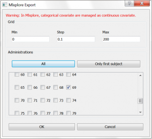
In this part, we would like to explore the influence of the parameters of a 2-compartment model. From the Monolix GUI, where we have selected a (V,k,k12,k21) model from the PK library, we have clicked on the blue icon to open Mlxplore. In the pop-up window, we can choose which individual we would like to simulate. We choose individual 69, which has only a few doses administrated, and modify the time grid to 0:0.1:200 as shown below:
In the Mlxplore application that has opened, a script has been automatically generated to define the simulation to run. The script contains information about:
- the data file, to overlay the data on top of the simulation
- the model, with its longitudinal part (structural model (V,k,k12,k21) from the library), the covariates, and the distributions for the individual parameters
- the parameter values, taken from the Monolix GUI and the covariates taken from the data set
- the administrations, with time and amount information, taken from the data set for individual 69
- the output to display, and the time grid
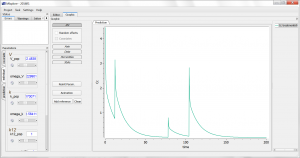
This script is editable, but let’s first run it as is, by clicking the blue arrow run button. The simulation is displayed. One sees the 4 administrations of different doses, and the non-linearity during the elimination phase. Using the sliders on the left, one can observe the influence of the parameter values on the simulation. Clicking the “Add reference” button permits to freeze a curve to better compare.
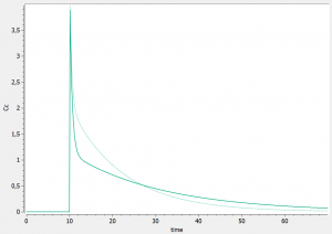
As having several doses is not very convenient, we can go back to the editor tab and modify the [ADMINISTRATION] subsection to
adm1_1={ type=1,time={10}, amount={100} }
such that only one dose at time 10 and of amount 100 is administrated. We also modify the time grid to
grid=0:0.1:70
and run the model again. For instance, the influence of reducing the value of k21 (dark curve versus light curve) can well be understood:
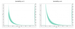
In addition to the individual parameters, the inter-individual variability (iiv) can also be visualized. In order to explore the impact of the iiv for each parameter individually, we first set all omega_* values to 0, except for the volume V. We then tick the “Random effects” box in the IIV tab. The prediction distribution is displayed, and one can see that the inter-individual variability on V will mainly influence the maximal level after the bolus dose. On the contrary, inter-individual variability on k has more impact at intermediate times after the dose:
One can also go to the “covariate” tab on the left, and play with the covariate values to see their impact on the simulation.
To change percentile levels, colors, labels, scales, etc look into the various menu tabs. To change the sliders limits, click on the sprocket.
With Mlxplore we have better understood the influence of the parameters, and the influence of the inter-individual variability.
Next part: Simulations for individualized dosing with Simulx and Monolix