Introduction
The purpose of this case study is the exploration of a tumor growth inhibition model for low-grade glioma treated with chemotherapy or radiotherapy. The model has been published in Ribba et al. in Clinical Cancer Research (18(18); 5071–80). The research goal is to describe the tumor size evolution in patients treated with chemotherapy or radiotherapy, and to explore the impact of treatments on the tumor growth, along with the impact of inter-individual variability.
Tumor growth inhibition model
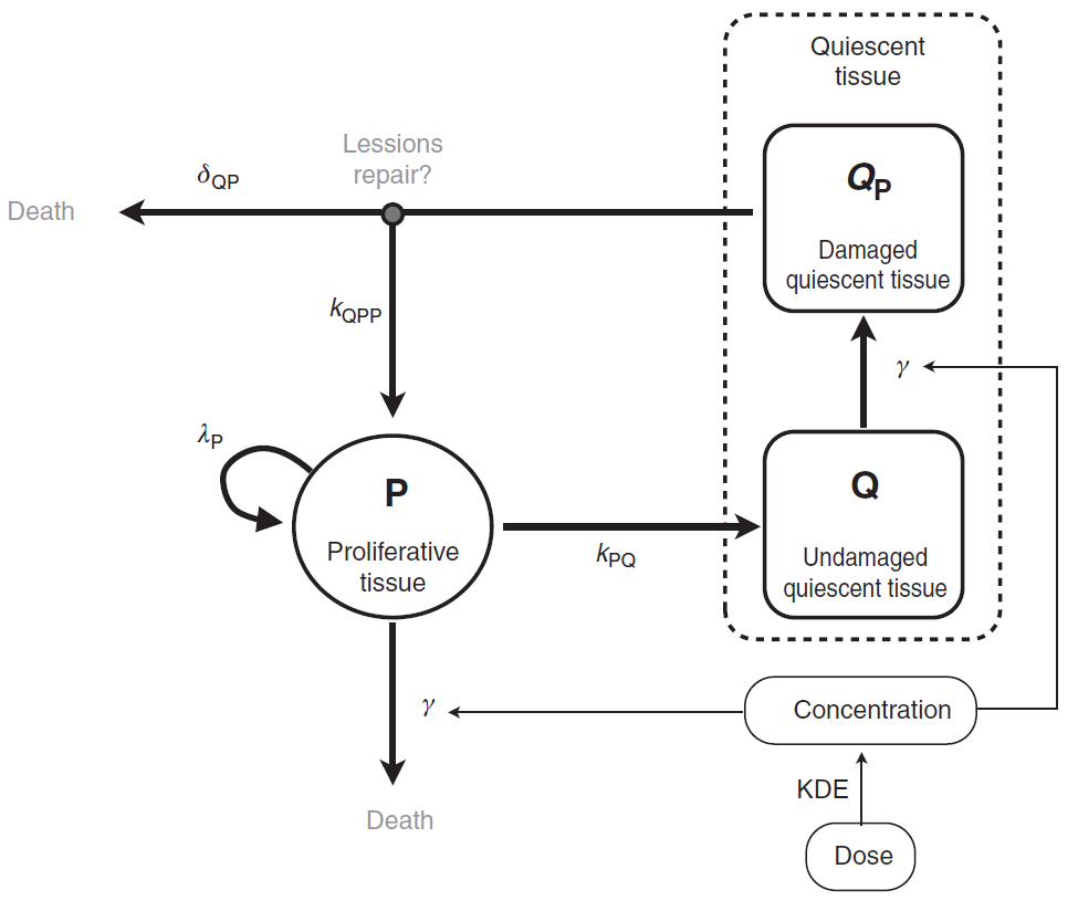
The tumor is composed of proliferative (P) and nonproliferative quiescent tissue (Q), expressed in millimeters. The transition of proliferative tissue into quiescence is governed by a rate constant denoted 

The pharmacokinetics of the PCV chemotherapy is modeled using a PK/PD approach, in which drug concentration is assumed to decay according to an exponential function. In this model, the three administrated drugs were not considered separately. Rather, the authors assumed the treatment to be represented as a whole by a unique variable (C), which represents the concentration of a virtual drug encompassing the 3 chemotherapeutic components of the PCV regimen. Following Ribba et al., the model writes
+k_{Q_{P}P}\times Q_{P}-k_{PQ}\times Q - \gamma_{P} KDE \times C \times P\\\frac{dQ}{dt} = k_{PQ}P-\gamma_Q \times C \times KDE \times Q \\\frac{dQ_{P}}{dt} = \gamma_{Q}\times C \times KDE \times Q - k_{Q_{P}P}Q_{P}-\delta_{QP}\times Q_{P}\\P^{\star} = P+Q+Q_{P}\end{array}\right.")
Notice that, in the publication, 
 = 0 \\P(t=0) = P_{0}\\Q(t=0) = Q_{0}\\Q_{P}(t=0) = 0\end{array}\right.")
A schematic view of the model proposed in Ribba et al. is represented here:
How to model it in Mlxtran
The purpose here is to define the model in Mlxtran language. The model writes as 4 ODEs. The resulting set of parameters is ")
")
[LONGITUDINAL]
input={lambdaP, kPQ, kQPP, gamma, deltaQP, KDE, P0, Q0}
Then, we start the EQUATION: block with the initial conditions:
EQUATION:
; definition of the initial time
t_0 = 0
; initialization of the ODEs
P_0 = P0
Q_0 = Q0
C_0 = 0
QP_0 = 0
and continue it with the 4 ODEs and the definition of

K = 100
PSTAR = P+Q+QP
ddt_C = -KDE*C
ddt_P = lambdaP*P*(1-PSTAR/K) + kQPP*QP - kPQ*P - gamma*P*KDE*C
ddt_Q = kPQ*P - gamma*Q*KDE*C
ddt_QP = gamma*Q*KDE*C - kQPP*QP - deltaQP*QP
The individual parameters corresponding to the 8 population parameters (6 parameters and 2 initial conditions) were assumed to be log normally distributed across individuals. Therefore, we have to define an [INDIVIDUAL] subsection as follows:
[INDIVIDUAL]
input = {lambdaP_pop, kPQ_pop, kQPP_pop, gamma_pop, deltaQP_pop, KDE_pop, P0_pop, Q0_pop,
omega_lambdaP, omega_kPQ, omega_kQPP, omega_deltaQP, omega_KDE, omega_P0, omega_Q0}

DEFINITION:
lambdaP = {distribution = lognormal, typical = lambdaP_pop, sd = omega_lambdaP}
kPQ     = {distribution = lognormal, typical = kPQ_pop,     sd = omega_kPQ}
kQPP    = {distribution = lognormal, typical = kQPP_pop,    sd = omega_kQPP}
gamma   = {distribution = lognormal, typical = gamma_pop,   sd = omega_gamma}
deltaQP = {distribution = lognormal, typical = deltaQP_pop, sd = omega_deltaQP}
KDE     = {distribution = lognormal, typical = KDE_pop,     sd = omega_KDE}
P0  = {distribution = lognormal, typical = P0_pop,          sd = omega_P0}
Q0  = {distribution = lognormal, typical = Q0_pop,          sd = omega_Q0}
The model is then the sum of all these codes and is implemented in TumorGrowthInhibitionModel_mlxt.txt
Model and treatment exploration: project definition
To define the project, we must define the model (in the <MODEL> section, as done in the previous paragraph), all parameter values (for the *_pop and omega_*, in the <PARAMETER> section) and the output (name and time grid, in the <OUTPUT> section). To explore the model, we define in the section <DESIGN> three administrations where we vary the inter dose timing and keep the same annual amount.
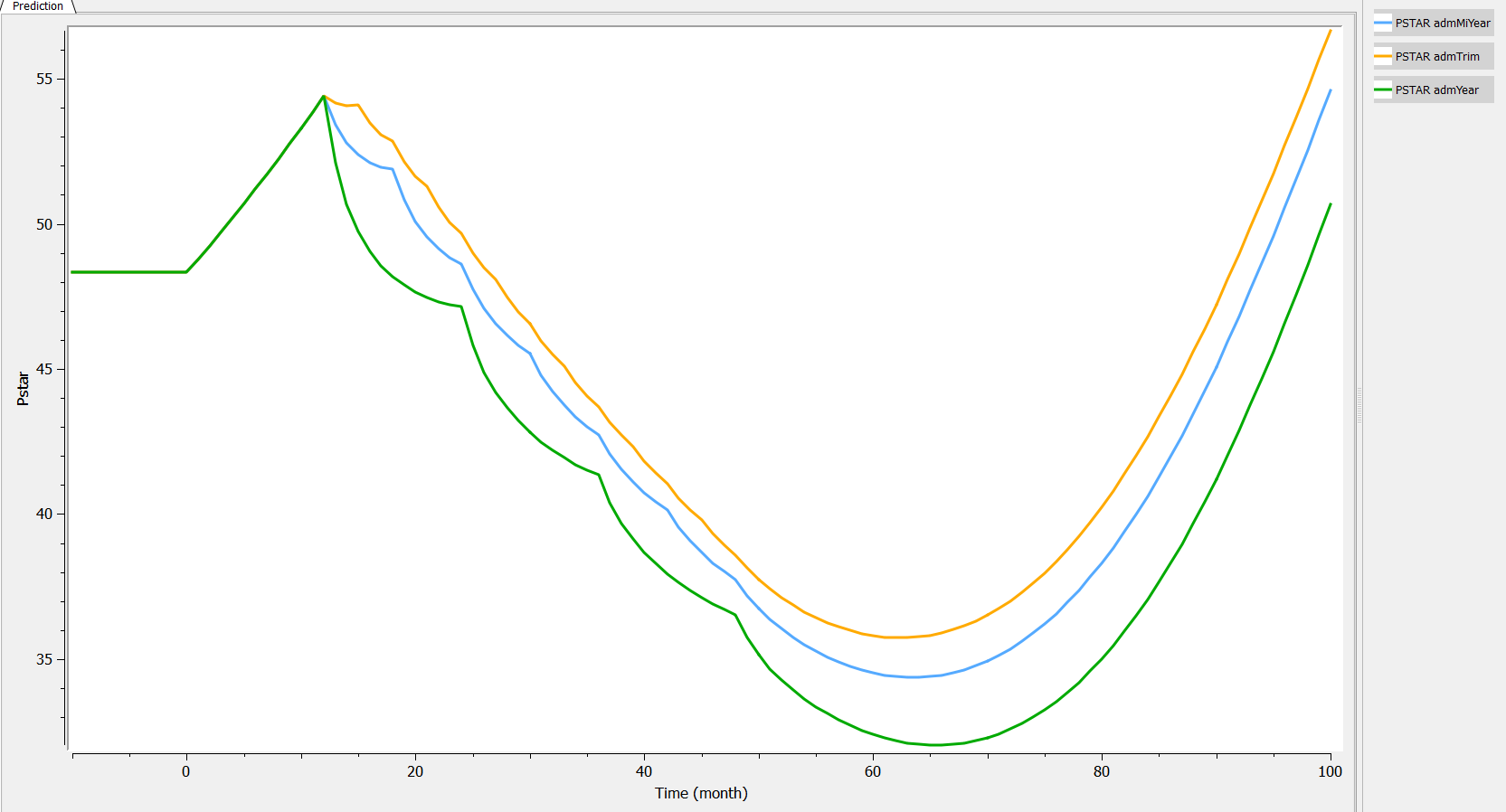
- “admYear”, where we administrate an amount of 2 each 12 months starting after 12 months
- “admMiYear”, where we administrate an amount of 1 each 6 months starting after 12 months
- “admTri”, where we administrate an amount of .5 each 3 months starting after 12 months
Finally, a section is added to define the graphic we want to look at. Then, the project is implemented in TumorGrowthModel_mlxplore.txt as follows:
<MODEL>
file = './TumorGrowthInhibitionModel_mlxt.txt'

<DESIGN>
[ADMINISTRATION]
admYear = {time=12:12:48, amount=2, target=C}
admMiYear = {time=12:6:48, amount=1, target=C}
admTrim = {time=12:3:48, amount=.5, target=C}

<PARAMETER>
; Parameters for the PCV treatment
lambdaP_pop = 0.121
kPQ_pop = 0.0295
kQPP_pop = 0.0031
gamma_pop = 0.729
deltaQP_pop = 0.00867
KDE_pop = 0.24
P0_pop = 7.13
Q0_pop = 41.2

omega_lambdaP = .03
omega_kPQ = .03
omega_kQPP = .03
omega_deltaQP = .03
omega_KDE = .03
omega_P0 = .03
omega_Q0 = .03

<OUTPUT>
list = {PSTAR}
grid = -10:1:100

<RESULTS>
[GRAPHICS]
pstar = {y={PSTAR},  ylabel = 'Pstar', xlabel = 'Time (month)'}
Model exploration: graphical results
Two aspects can be analyzed: the predictions and the inter-individual variability. First we can explore the predictions associated with the three kinds of administrations:
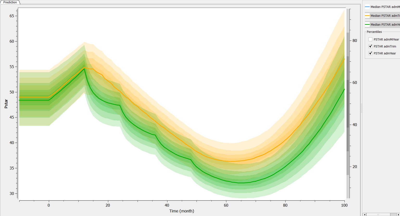
Then, if one wants to explore the impact on the inter-individual variability, one can click on iiv leading to the following figure:
Conclusion
In this example, a relatively complex ODE model has been implemented in Mlxtran, and its behavior (predictions following different treatments, as well as inter-individual variability) as been explored with Mlxplore.