Using delays, the example of rheumatoid arthritis

Introduction

Rheumatoid arthritis (RA) is an immune-mediated inflammatory disease and is characterized by a chronic inflammation and synovial hyperplasia leading to the destruction of cartilage and bone. Approximately one percent of the world-wide population suffers from RA. The model is presented in a poster published at PAGE in 2011 by Gilbert Koch. The research goal is to develop a multi response model to describe the time course of the total arthritic score and the strongly delayed ankylosis score measured in collagen induced arthritic (CIA) mice. The authors used a three compartment delay differential equation model to get a deeper understanding between cytokine level, inflammation and bone destruction.

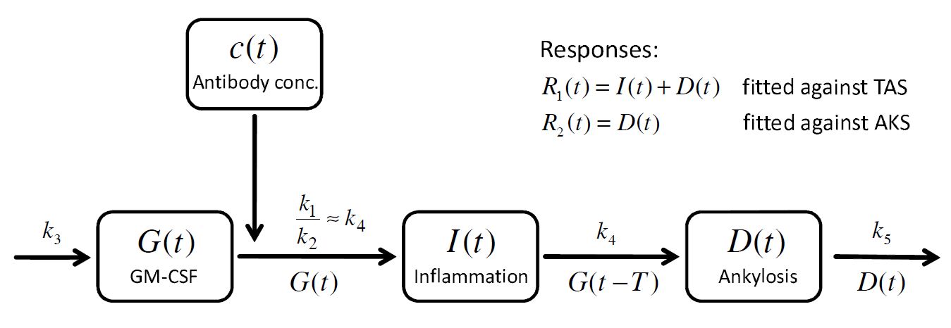
A multi-response model for rheumatoid arthritis

The modeling part was done in three steps. We will follow the steps presented by Koch in his PhD thesis.

Modeling Step 1: The cytokine behavior in time.
The cytokine GM-CSF (noted $G$ ) drives the disease. Its kinetics is described by:

$\frac{dG}{dt} = k_3-\frac{k_1}{k_2}(1-e^{-k_2t})G(t) - E(Cc(t))G(t)$

The last term models the effect (function $E$ ) of the anti-GM-CSF antibody concentration ( $Cc$ ) on the cytokine GM-CSF level $G$ . The effect of the antibody is described by the following expression: $E(Cc)=(\sigma_1*\exp(- \sigma_2*Cc) + \sigma_3)*Cc$ .

The concentration of the anti-body is described by a 2 compartment model with bolus administration and linear elimination.

Modeling Step 2: Multi-response approach to model the TAS and AKS
The mathematical model of the arthritic disease is split into an inflammatory part $I(t)$ and an ankylosis (bone and cartialge destruction) part $D(t)$ and the sum $R_1(t) = I(t) + D(t)$ defines the response $R_1(t)$ , which corresponds to the experimentally measured total arthritic score (TAS). In addition a second response function is defined as $R_2(t) = D(t)$ which corresponds to the ankylosis score (AKS).
To build a model for the time course of the inflammation $I(t)$ and the ankylosis $D(t)$ , the concept of lifespan modeling is introduced: the overall inflammation $I(t)$ is controlled by two processes, the inflow $k_{in}(t)$ and the outflow $k_{out}(t)$ . Assuming that the inflammation caused by these processes remains a certain time period $\tau$ and is driven by the amount of GM-CSF, one obtains $k_{out}(t) = k_{in}(t-\tau)$ and $k_{in}(t) = k_4 G(t)$ where $k_4$ is a first order rate constant. Then the total balance equation for the inflammation reads:

$\frac{dI}{dt} (t) = k_4G(t) - k_4G(t - \tau)$

Similarly, for the ankylosis $D(t)$ one obtains $k_{in}(\textrm{ankyloses}) = k_{out}(\textrm{inflammation})$ . Applying a first order loss term $k_{out}(\textrm{ankyloses}) = k_5D(t)$ leads to the equation:

$\frac{dD}{dt} (t) = k_4G(t-\tau) - k_5G(t)$

The presence of $G(t)$ and $G(t - \tau)$ reflects that the inflammation and the ankylosis are driven by GM-CSF. Moreover, the action of GM-CSF on the ankylosis is delayed by $\tau$ . A schematic view of the model, proposed in Koch’s PhD thesis, is given here:

ArthritisSchematic

How to model it in Mlxtran

The purpose here is to define the model in Mlxtran language. The system writes as a PKPD model with a DDE. The resulting set of parameters is (alpha, beta, CL, V1, V2) for the PK model, (sigma1, sigma2, sigma3) for the effect model, and (k1, k2, k3, k4, k5, tau) for the RA model along with 3 additional initial conditions (I0, a,b). Therefore, the [LONGITUDINAL] subsection starts with:

[LONGITUDINAL]
input = {a, b, I0, alpha, beta, CL, V1, V2, sigma1, sigma2, sigma3, k1, k2, k3, k4, k5, tau}

Then, we start the EQUATION: block with the initial conditions:

EQUATION:
; initialization of the time
t0 = 0

; initialization of the variables of interest
I_0 = I0
D_0 = 0
G_0 = a*exp(b*t)

Notice that the initialization of the variable G is not only at time 0 but also across the past $[-\tau, 0]$ . One continues with the PKPD model:

K12 = alpha*beta*V2/CL
K21 = alpha*beta*V1/CL
Cc = pkmodel(k12=K12,k21=K21,V=V1,Cl=CL)
E = (sigma1*exp(- sigma2*Cc) + sigma3)*Cc

and the ODE/DDE equations along with the definition of the TAS and the AKS:

ddt_G = k3 - E*G - (k1/k2)*(1- exp(- k2*t))*G
ddt_I = k4*G - k4*delay(G,tau)
ddt_D = - k5*D + k4*delay(G,tau)

TAS = I+D
AKS = D

Finally, the individual parameters representing the variability of the delay are defined as a normal distribution and one writes:

[INDIVIDUAL]
input = {tau_pop, omega_tau}

DEFINITION:
tau = {distribution = normal, mean = tau_pop, sd = omega_tau}

The model is then the sum of all this code and is implemented in arthritisModel_mlxt.txt

Model and treatment exploration: project definition

To define the project, one must define the model (done in the previous paragraph, section <MODEL>), the parameter values (section <PARAMETER>) and the output (section <OUTPUT>). To explore the model, we define in the section <DESIGN> three administrations where we vary the amount of antibody.

“Trt_0”, where we administrate nothing
“Trt_1”, where we administrate 1 mg/kg (and thus 70mg) each week during 5 weeks
“Trt_1”, where we administrate 10 mg/kg (and thus 700mg) each week during 5 weeks

Finally, a section is added to define the graphics we want to look at. The project is implemented in arthritisModel_mlxplore.txt as follows

;model definition
<MODEL>
file='./arthritisModel_mlxt.txt'

<DESIGN>
[ADMINISTRATION]
trt_0 = {time = {1, 8, 15, 22, 29}, amount = 0}
trt_1 = {time = {1, 8, 15, 22, 29}, amount = 70}
trt_10 = {time = {1, 8, 15, 22, 29}, amount = 700}

;parameter initial values
<PARAMETER>
; Initialization parameters
a = 1
b = 0.5
I0 = 2.52

; PK model 
alpha = 0.02327
beta = .045
CL = 2.5
V1 = 15
V2 = 25

; Effect model 
sigma1 = 0.154
sigma2 = 0.065
sigma3 = 0.003

; Arthritis model parameters
k1 = 0.183
k2 = 0.092
k3 = 5
k4 = 0.064
k5 = 0.016
tau_pop = 11.2
omega_tau = 3

;prediction outputs and grid
<OUTPUTS>
list={TAS,AKS, G, I, D,Cc}
grid=0:.01:40

<RESULTS>
[GRAPHICS]
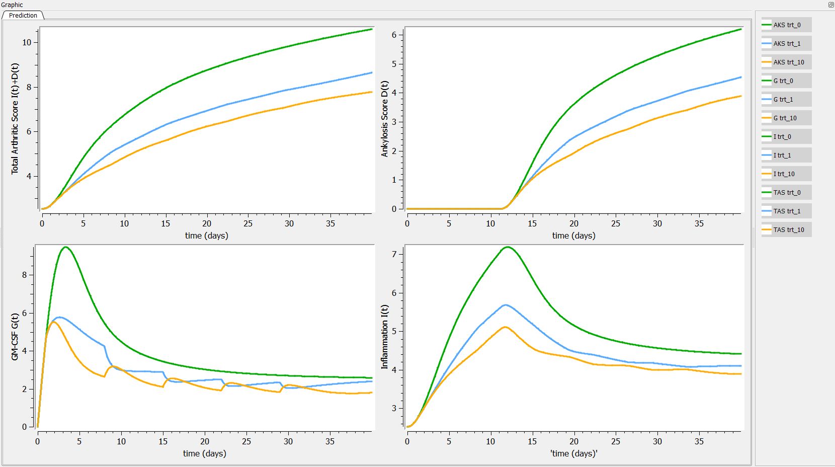
pTAS = {y={TAS},  ylabel = 'Total Arthritic Score I(t)+D(t)', xlabel = 'time (days)'}
pAKS = {y={AKS},  ylabel = 'Ankylosis Score D(t)', xlabel = 'time (days)'}
pG = {y={G},  ylabel = 'GM-CSF G(t)', xlabel = 'time (days)'}
pI = {y={I},  ylabel = 'Inflammation I(t)', xlabel = 'time (days)'}
gridarrange(pTAS, pAKS, pG, pI, 2,2)

<SETTINGS>
[GRAPHICS]
nb_simulations = 200

Model exploration: graphical results

First we can explore the predictions following the 3 different treatments:

Arthritis
Then, if one want to explore the impact on the inter-individual variability on the delay, one can click on iiv leading to the following figure:

ArthritisDelay

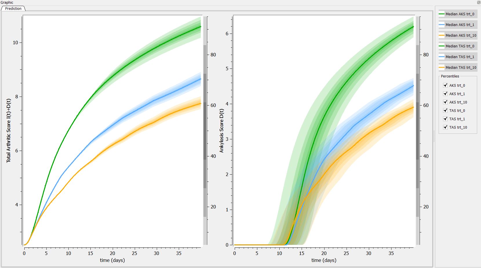
Conclusion

In this example, we have implemented a model with ODEs, and DDEs with complex initial conditions using Mlxtran. Using Mlxplore, we have explored the influence of different treatments on the predictions. Mlxplore also enables to visualize the inter-individual variability.