1.Home
Version 2019
This documentation is for Monolix Suite 2016 and later.
©Lixoft
Mlxplore is an application for the visual and interactive exploration of your models, designed to be intuitive and easy to use. It is a powerful solution for daily modeling work as well as for teaching and sharing PK/PD properties or for real time dose-regimen exploration in front of an audience. Mlxplore also allows you to visualize the statistical components of the model, such as the impact of covariates and inter-individual variability.
Mlxplore main window
Easy model implementation
Mlxtran is used for custom-built models; a simple, yet powerful model language that is suitable for simple PK as well as complex Systems Pharmacology models. Mlxtran contains a set of macros and keywords for PK/PD models.
Simple implementation of study design
Treatments and administrations are specified as Mlxtran code.
Powerful user-friendly interface
Mlxplore offers an easy-to-use, flexible and fully interactive interface. It contains an embedded text editor with auto-help and syntax highlighting for Mlxtran language and Mlxplore projects.
Fast computing of complex models
Models are automatically compiled in the background for lightning fast simulations. Mlxplore includes an efficient ODE solver, as well as a solver for delayed differential equations (DDE).
2.Mlxplore project construction
Introduction
Mlxplore projects for model exploration describe several elements in addition to the model itself. These include the administrations and treatments, the parameter values, the variables of interest for the graphics, and optionally some options for the graphics. These elements are defined in a text file, which is compiled to generate the graphics. Most of the model exploration can then be done in the GUI, via sliders and settings.
To define the Mlxplore project file, the user is recommended to start from demo projects included in the Mlxplore demos folder, which can be easily edited for custom user needs. Alternatively Mlxplore projects can also be created via an export from Monolix.
Overview of the project file architecture
The project file is structured in sections (<SECTION>) and subsections ([SUBSECTION]), which are detailed below:
- section <MODEL> (mandatory): this section defines the model, including its structural and statistical elements. Most of the time, the model is defined in a separate file, and the Mlxplore project file only provides the path to it, e.g
file='path/model.txt'. In the model file, the model is defined via the subsections [LONGITUDINAL] (mandatory), [INDIVIDUAL] (optional) and [COVARIATE] (optional), as detailed in the mlxtran documentation. A detailed description of the three mandatory sections is given here.
- section <DESIGN> (optional): in this section, the amount, target/type and time schedule of the administrations are defined in the [ADMINISTRATION] subsection. Treatments (i.e combinations of administrations) can be defined in the [TREATMENT] subsection. More details about the definition of administrations and treatments are given here.
- section <PARAMETER> (mandatory): in this section the parameter values used as reference values for the simulations are defined. The parameters defined in the
input={...}lines of the [LONGITUDINAL], [INDIVIDUAL] and/or [COVARIATE] model subsections must be set (if not defined by another model subsection). A detailed description of the three mandatory sections is given here.
- section <OUTPUT> (mandatory): in this section, the variables to display (e.g
list={Cc,Ce}) and the time points at which the model will be simulated (e.ggrid=0:0.05:10) are defined. A detailed description of the three mandatory sections is given here.
- section <RESULTS> (optional): in this section, in the subsection [GRAPHICS], the graphics to display can be pre-defined, while full options are available via the GUI. More details about the definition of the graphics are given here.
- section <SETTINGS> (optional): in this section, in the subsection [GRAPHICS], the settings for the simulations (such as the number of simulations for the iiv) can be defined. More details about the definition of the settings are given here.
2.1.What is mandatory ?
Introduction
Different components of the model are implemented in different sections. To run, a project must have at least:
- a section <MODEL> that defines the model you want to explore. This section contains at least the structural model but can also contain the inter-individual variability and the covariates definition. To see how to build a model in Mlxtran, click here.
- a section <PARAMETER> that defines the parameters used in the model, and which value will be available in the graphical interface as sliders.
- a section <OUTPUT> that defines the variables that you want to look at and the time points at which the model will be simulated.
To show exactly how to define it, let’s see the following example. This example is meant to show the general structure, while the construction on the model will be detailed in the following sub-section of this user guide.
Example
Here is a very simple example where we want to explore a simple linear equation of the form y=at+b where t is the time and a and b are parameters. First, we have to define the model. For that, we use the section <MODEL> and define the model in the [LONGITUDINAL] subsection. The construction of a [LONGITUDINAL] section is defined in the Mlxtran documentation here. In the project, it should be written in the following form:
<MODEL>
[LONGITUDINAL]
input = {a,b}
EQUATION:
y = a*t+b
Second, we have to define the parameters we are gonna play with and their reference value. In that case, two parameters a and b with initial conditions a=1 and b=2 write:
<PARAMETER>
a = 1
b = 2
Finally, we have to define the output we would like to display. Both names (through a list) and the timing have to be defined.
<OUTPUT>
list = {y}
grid = 0:.1:100
Notice that an input parameter of block ([INDIVIDUAL] and [LONGITIDINAL]) can not be used as an output.
At the end, to full project looks like that:
<MODEL>
[LONGITUDINAL]
input = {a,b}

EQUATION:
y = a*t+b

<PARAMETER>
a = 1
b = 2

<OUTPUT>
list = {y}
grid = 0:.1:100
The best practices associated with the model definition and implementation in the <MODEL> section are largely detailed in other sections of this documentation. Therefore, we focus here on the <PARAMETER> and <OUTPUT> sections.
Best practices for <PARAMETER> section
- If a parameter is not used in the model but defined in the subsection <PARAMETER>, the exploration will run but a warning saying that “a parameter ‘unused_param’ is not defined in the model”.
- No computation is allowed in the <PARAMETER> section. Therefore,
a=1+2is not possible, it has to be a numerical value. - No identification is allowed in this section. Therefore,
<PARAMETER>
a = 1
b = a
is not allowed. If such identification is needed, it can be done directly in the model.
Best practices for <OUTPUT> section
- The grid definition represents the time where the user will see the outputs. The ODE/DDE solver may evaluate the model at shorter time intervals.
- Several outputs can be considered. They have to be listed in the list of the section <OUTPUT> , for example
list={output1, output2, ...}. All the outputs will share the same time grid. - If an output of the list has not been previously defined, an error will occur and is explicitly displayed to the user.
- The grid has not to be regular. One can define explicitly the grid, for example
grid={t_1, t_2, ..., t_n}. We strongly recommend to define the timest_ias a strictly increasing suite for readability. - An hybrid version of the grid definition such as
grid={t_1a:dt_a:t_Na, t_1b:dt_b:t_Nb}is not supported and generates errors.
2.2.Administration and treatment design
By administration, we refer to one or several dose administrations via the same route (iv, oral, etc). The times, amounts, rates and the target or administration adm identifier can be defined by the user. By treatment, we refer to a combination of elementary administrations. Both administrations and treatments are defined in the <DESIGN> section.
Definition of administrations
Introduction
To explore treatments in MlxPlore, the user can define drug administrations. It must be implemented in the subsection [ADMINISTRATION] in the section <DESIGN>. The goal is to be able to define, the time(s), the amount(s), the rate(s), and the type or the target of the administration. Here is the way to define all these parameters :
- Timing: The drug administration’s time(s) are defined by the keyword
time. You can define either a single time withtime=0or a list of times withtime={0,2,6}for irregularly spaced doses ortime=1:2:7(without curly braces) for regularly spaced doses. - Amount: The drug’s amount is defined by the keyword
amount. If the amount is the same for all times, you can give the amount only once asamount=100. To define a different dose for each time, use a list asamount={100, 50, 25}. - Infusion rate/duration: The drug’s administration rate (if applicable) is defined by the keyword
rate. The rate corresponds to the speed of administration. Thus, for a given rate, the drug is administrated during a time tinf=amount/rate. Theratekeyword is optional. If not defined, the rate is infinitely fast, which corresponds to a bolus administration. Instead of the administration rate, the administration duration can also be given, using the keywordtinf. Again, either single values or a list can be given, for instance:rate=2.5,rate={7,10},tinf=40,tinf={1,4,9,10}. - Target/administration identifier: The target of the administration is defined by the keyword
target. It corresponds to the name of the component of the ODE system that receives the input. When using administrations on ODEs, you have to make sure the target is one of the variable into consideration. If the target does not correspond to a component, then the administration does not occur. Alternatively, the user can define an administration identifier via the keywordtype. The administration is then associated with the administration macro of the model having the same identifier. One could for instance writetarget=Acortype=1. Lists are not allowed for target and type, yet the treatments allow to define combinations of administrations.
Examples of the <DESIGN> section
<DESIGN>
[ADMINISTRATION]
admin1 = {time=5, amount=1, target=Ad}
admin2 = {time=0:1:10, amount=1, type=1, rate = 0.5}
admin3 = {time={0,5,7}, amount={10,15,10}, target=Ad, tinf=1}
Example of a full Mlxtran file for Mlxplore
To illustrate an administration, we propose an example of a one compartmental model with a first order absorption model (with an absorption rate ka) and a linear elimination (with a clearance Cl from the central compartment) and several types of administration (bolus and infusion). The amount of drug in the depot compartment is denoted Ad, while the amount in the central compartment of volume V is Ac. We look at the concentration Cc=Ac/V in the central compartment as an output. This model is implemented in the file singledose.mlxplore.mlxtran
<MODEL>
[LONGITUDINAL]
input = {ka, V, Cl}

EQUATION:
t0 = 0
Ad_0 = 0
Ac_0 = 0

ddt_Ad = -ka*Ad
ddt_Ac = ka*Ad -Cl/V*Ac
Cc = Ac/V

<DESIGN>
[ADMINISTRATION]
admin_bolus    = {time=5, amount=1, target=Ad}
admin_infusion = {time=5, amount=1, target=Ad, rate = 0.5}

<PARAMETER>
ka = 1
V = 10
Cl = .5

<OUTPUT>
grid = 0:.05:20
list = {Cc}
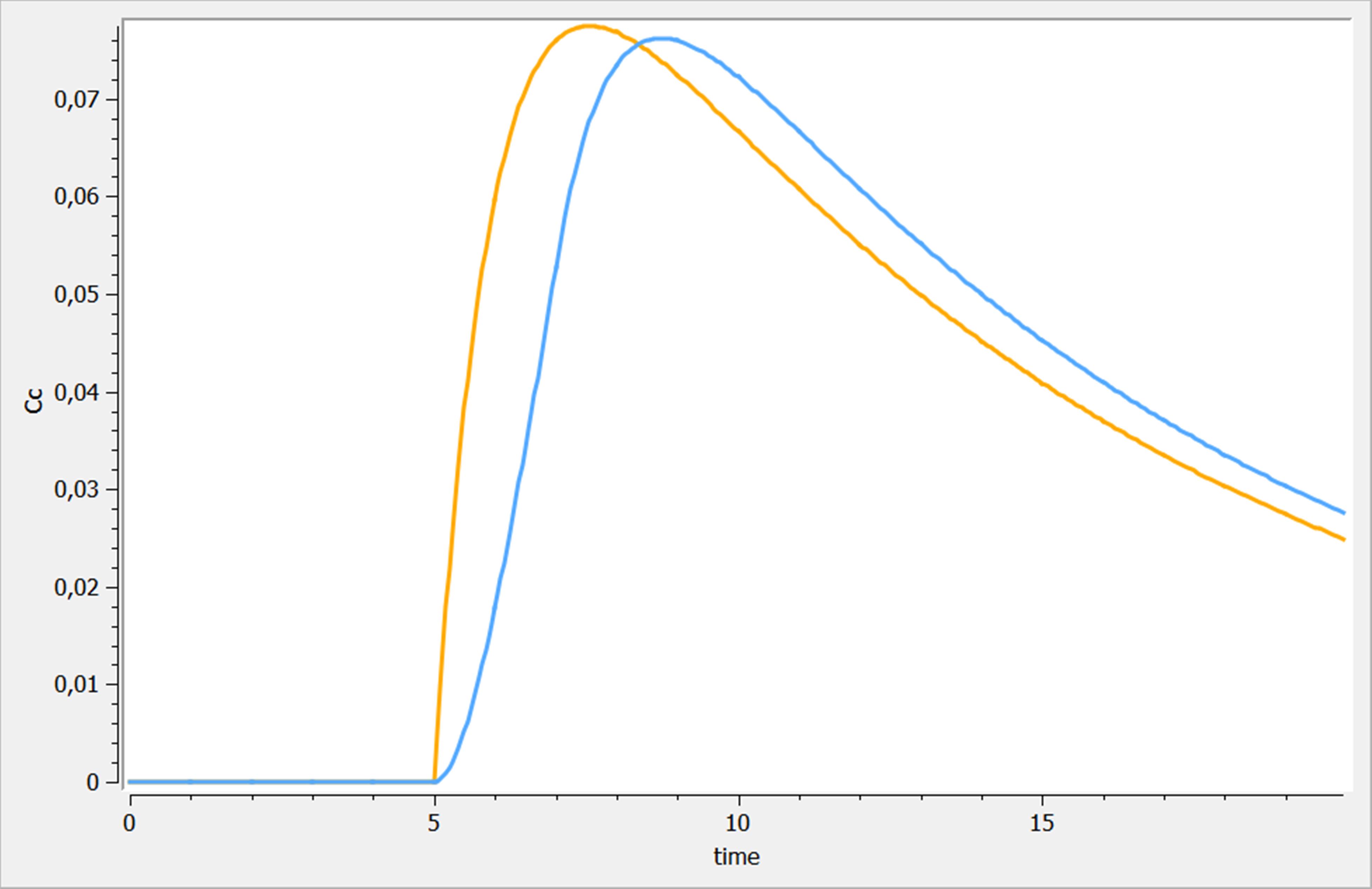
The results of the exploration of this model are presented in the following figure. We can see the two different administrations and the impact of the rate on the output. The “admin_bolus” is displayed in orange, while the “admin_infusion” is displayed in blue.
Best practices
- No computation in the definition of the administration is allowed. It is then not possible to define an amount with a sum (ex.
amount=1+1oramount=1*2). The same applies for the other keywords. - When defining the times as
time=t1:dt:tn,dtmust be strictly positive. - If the
amount,rateortinfis defined via a list, the length of the list must agree with the number of doses defined with thetimekeyword. - The definition of
rateandtinfare mutually exclusive. - The definition of
targetandtypeare mutually exclusive. - The identifiers following the
typekeyword should be integers.
Best practices Ex. 1 : Variations on multiple dosing
Three variations of multiple dosing are used in the following example, where the same model is used. This model is implemented in the file mlxplore_multipledose.txt and the only difference with the previous example is the [ADMINISTRATION] subsection, where the previous administration is replaced by
[ADMINISTRATION]
adm_t = {time={2, 7, 12}, amount=1, target =Ad, rate=1}
adm_t_am = {time={2, 7, 12}, amount={1,1,1}, target =Ad, rate=.5}
adm_t_am_rate = {time=2:5:15, amount={1,1,1}, target =Ad, rate = {4, 2, 1}}
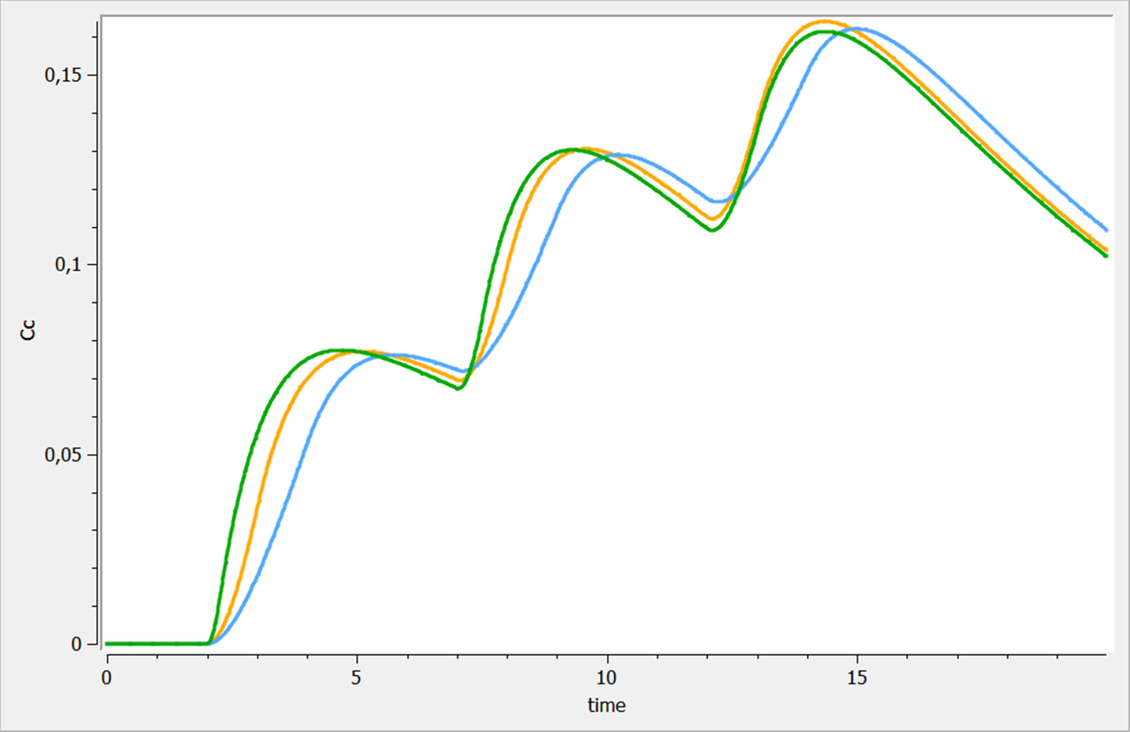
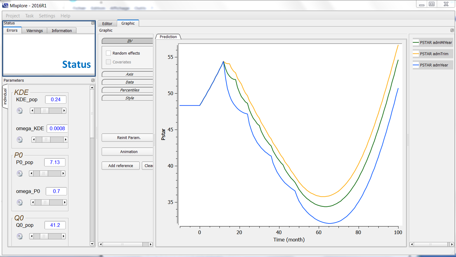
The three results are shown on the following figure. adm_t, adm_t_am and adm_t_am_rate are presented in blue, orange and green respectively.
Definition of treatments
Introduction
A treatment is a combination of administrations, such that administrations needs to be defined first, before treatments can be defined. Treatments must be implemented in the subsection [TREATMENT] of the section <DESIGN> of a script Mlxtran. Treatments are for instance useful if doses are administrated via different routes (iv, oral, etc) to an individual. In this case, you define first the administrations (iv and oral for instance) and then combine them in a treatment. The syntax is straighforward: treat1={adm1, adm2, ...}. The treatment section is optional.
Example
To illustrate the use of treatments, we reuse the same model as above.
In this example, three administrations are defined:
- admAd1 : unitary amount with target Ad, each 12h,
- admAd2 : twice the dosage of admAd1 but each 24h,
- admAc : amount of .25 in the central compartment for Ac each 24h,
and we combine the administrations in two treatments:
- trtRef : simply the administration admAd1
- trtComb : the combination of administrations admAd2 and admAc
With that definition, we are able to compare treatments that can have several dosages, timings, but more importantly targets and types. This model is implemented in the file mlxplore_treat.txt
<MODEL>
[LONGITUDINAL]
input = {ka, V, Cl}

EQUATION:
t0 = 0
Ad_0 = 0
Ac_0 = 0

ddt_Ad = -ka*Ad
ddt_Ac = ka*Ad -Cl/V*Ac
Cc = Ac/V

<DESIGN>
[ADMINISTRATION]
admAd1 = {time=0:12:168, amount=1, target=Ad}
admAd2 = {time=0:24:168, amount=1,  target=Ad}
admAc = {time=0:12:168, amount=.5,  target=Ac}

[TREATMENT]
trtRef = {admAd1}
trtComb = {admAd2, admAc}

<PARAMETER>
ka = .1
V = 10
Cl = 1

<OUTPUT>
grid=0:.05:168
list = {Cc}
The results of the treatments are proposed in the following figure. The treatment “trtRef” is in orange, while “trtComb” is in blue.
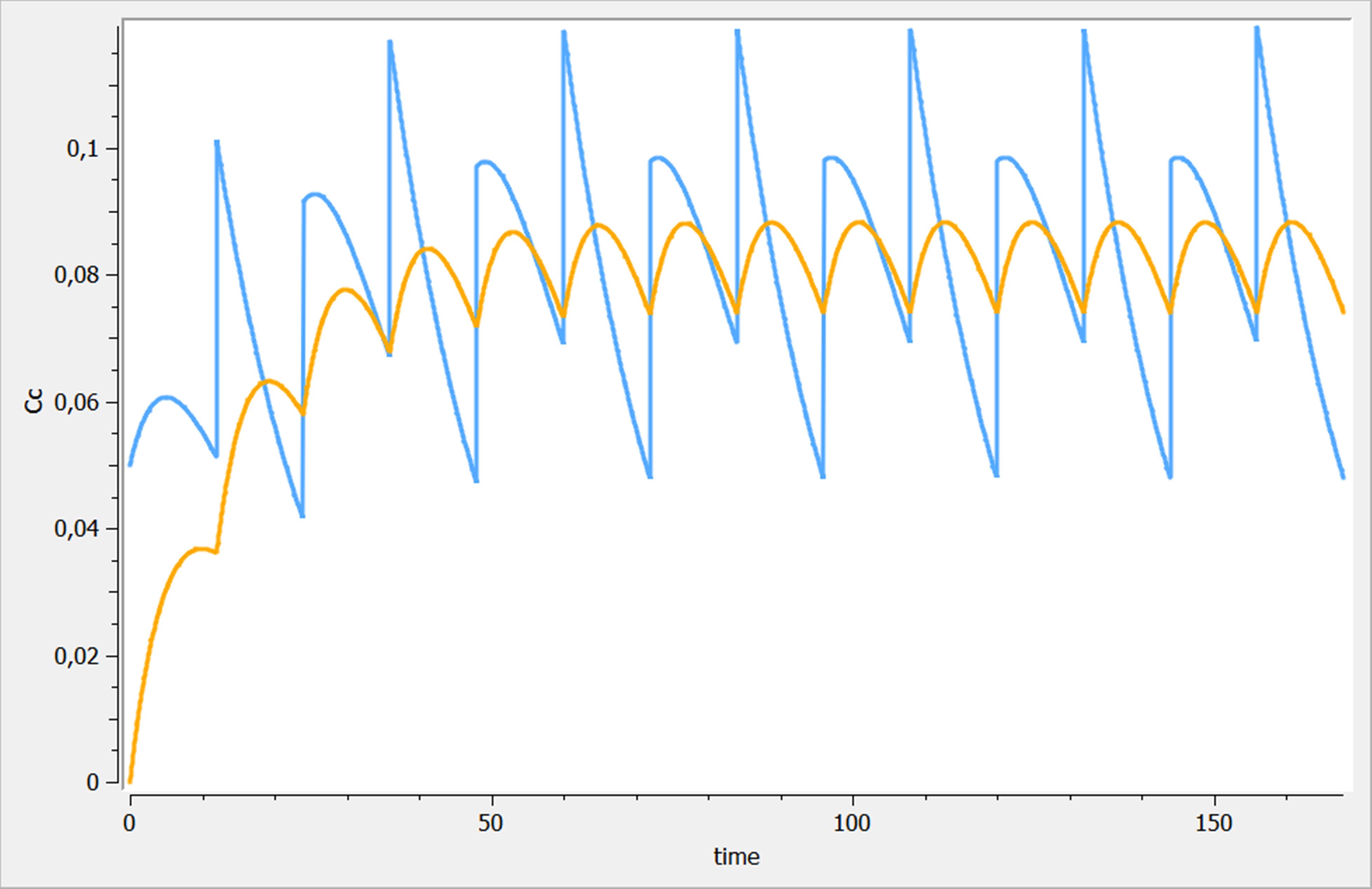
Best practices
- If no dedicated subsection [TREATMENT] is defined by the user, we define in the interface as many treatments as administrations and explore all of them.
- If a subsection [TREATMENT] is defined, and an administration is defined but not used in the treatments, this administration will not be applied.
- We advise our users to define all the administrations they want to explore and to define the subsection [TREATMENT] with a smaller number of treatments. Like that, you can explore each treatment and make your exploration much simpler.
2.3.Graphics
The section <RESULTS> permits to define the graphics to display. It is optional, and by default every output defined in the <OUTPUT> section will be plotted w.r.t time.
To pre-define the graphics, a section [GRAPHICS] is used with the following information:
- The output on the X-axis, using the keyword
x. If omitted, the value by default is the time. Any variable listed in the <OUTPUT> section can be used, for instancex={Ac}. - The output on the Y-axis, using the keyword
y, for exampley={Cc}. This is mandatory. Several outputs can be displayed on the same graph, for instance withy={Ac,Ad}. The outputs to display must be taken from the list of outputs defined in the <OUTPUT> section. - The label of the X-axis, using the keyword
xlabel. The desired xlabel should be specified under quotes, for instancexlabel='time (h)'. - The label of the Y-axis, using the keyword
ylabel. The desired ylabel should be specified under quotes, for instanceylabel='Concentration (mM)'.
These pre-defined graphics can be modified via the GUI later on. More options such as color, etc are then also available.
Example
If one wants to plot (Ad,Ac) w.r.t. time in a first plot and Ad w.r.t. Ac in a second plot, it writes in Mlxtran
<RESULTS>
[GRAPHICS]
p1 = {y={Ac,Ad}, ylabel='Ac,Ad', xlabel='Time'}
p2 = {y={Ad}, x={Ac}, ylabel='Ad', xlabel='Ac'}
Several graphics can be defined. To arrange them in space, the function gridarrange can be used. As arguments, the list of graphics to display is given, as well as the number of columns (e.g nb_cols=2, optional), and a flag to enforce the use of same y or x limits (samelimitsy=true and/or samelimitsx=true, optional). Thus, putting the two graphics, first p2 and then p1, in two lines with the same Y-axis writes:
<RESULTS>
[GRAPHICS]
p1 = {y={Ac,Ad}, ylabel='Ac,Ad', xlabel='Time'}
p2 = {y={Ad}, x={Ac}, ylabel='Ad', xlabel='Ac'}
gridarrange(p2,p1,nb_cols=1,samelimitsy=true)
2.4.Settings
Introduction
The graphics settings can be defined via the GUI, but most of them can also be defined in the project file, in the <SETTINGS> section. This is interesting for advanced users to pre-set the graphics.
IIV
To pre-define the activation/deactivation of the iiv sections, the user can define it in a section <SETTINGS> and a subsection [GRAPHICS]. For that, two keywords are used iiv_parameter and iiv_covariate. By setting them at true or false, you can directly define if the iiv computations should be performed when running the project. In Mlxtran, activating both of them writes:
<SETTINGS>
[GRAPHICS]
iiv_parameter = true
iiv_covariate = true
If no covariate is used in the model, and the setting is iiv_covariate=true, then obviously no drawing of the covariate is made and the checkbox in the user interface is grayed. The same is done for the individual parameters.
Percentile
To pre-define the values in the percentile tab, the user can define it in a section [GRAPHICS]. For that, three keywords are used: pred_interval, nb_band and nb_simulations for the level, the number of bands and the number of simulations respectively. In Mlxtran, defining 8 bands, a level of 90 with 200 simulations writes
<SETTINGS>
[GRAPHICS]
nb_simulations = 200
nb_band = 8
pred_interval = 90
3.Model exploration
Mlxplore has a graphical interface for model exploration using a project file. To explain the elements of the interface, a description of a typical example of a model and treatments exploration is used.
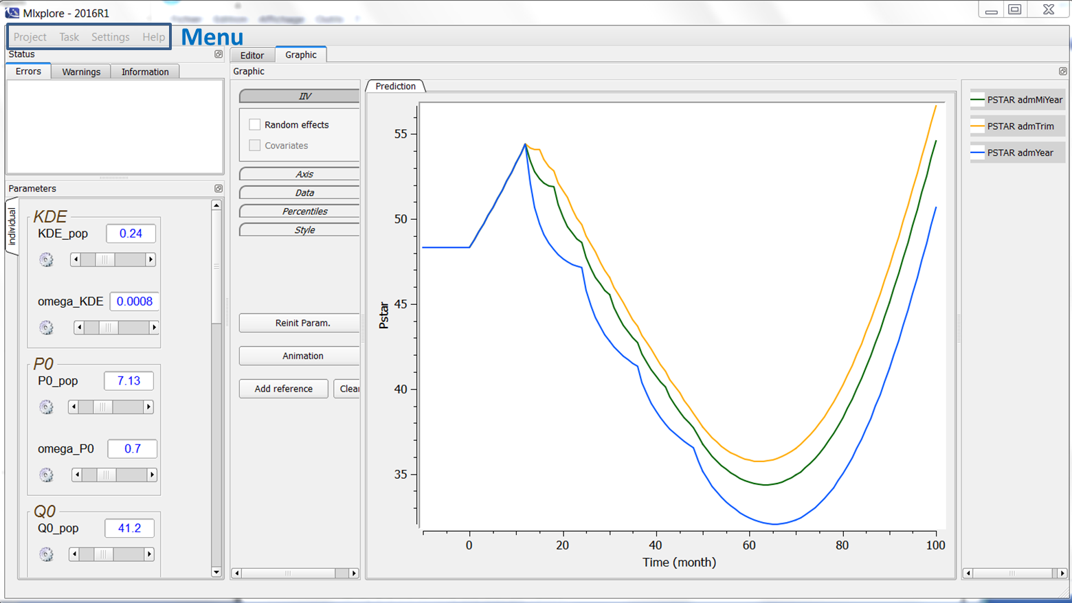
One can see four main areas in the Mlxplore GUI:
- The menu
- The parameters
- The graphics with the associated settings and legend
- The editors with the associated status.
3.1.Menu
Introduction
At the top of the Mlxplore main window, a menu bar is available, with submenus:
Project menu
The possible actions are defined in the following:
- “New”: creates a new project. There are three ways of creating a new project depending if you would like to define the model and the rest of the project separately or not. You can choose:
- “Model and Project in separated files”: In that case, the editor is split into two windows, one for the project and one for the model. This is particularly convenient when nothing is defined yet in your project. It allows you to work separately on the model construction and on the project definition. This is definitively the one we recommend.
- “Model embedded in the project”: In that case, only one window appears, to define both the project and the model. This is convenient when you want to have everything in the same file.
- “Project with existing model”: In that case, you load a model and two windows are created. One with the project and another one with the model you have chosen. This is particularly convenient when your model is already implemented and you want to explore it. Typically, this model comes from a Lixoft’s library or your own model library.
- “Load”: this allows you to load an existing project. If you try to load only a model file. A warning will appear. Notice that the user can load a project created by Monolix.
- “Save”: Saves the project.
- “Save as”: Saves the project as.
- “Close”: Mlxplore stays open but the current project is cleared.
- “Quit”: Quits Mlxplore.
- You can also load the past projects used by Mlxplore, that appear in the list.
Task
In this menu, you can:
- “Run”: run the project
- “Export figure”: export the figure. It can be done in .bmp, .jpg, or .png
- “Export table”: this exports a table of exploration results. A popup window appears to choose the folder. The table is saved as a .csv file with several columns. The columns are the ids, the times and the outputs.
- The id corresponds to the treatment number. If there are several treatments, they are defined in the table as several id (starting at id=1)
- The time is the time defined by the grid
- If no iiv is used, the output columns are the values w.r.t. time. If iiv is used, then each output is split in several values (the median and the percentiles defined by the number of band).
- “Export parameters”: this export a table of all the parameters. A popup window appears to choose the folder. The table is saved as a .csv file with two columns. The first one is the parameters name, and the second one the values.
Settings
In this menu, you can:
- “Display Editor”: Allow to hide/unhide the text editor window.
- “Display Status”: Allow to hide/unhide the status window (for errors and warnings).
- “Preferences”: Define the preferences (colors, fonts, etc) for the text editor, and choose the seed number.
Help
In this menu, you can click:
- “About”: gives the version of the software, along with the expiration date of the licence
- “Licence”: gives the terms of use of the software
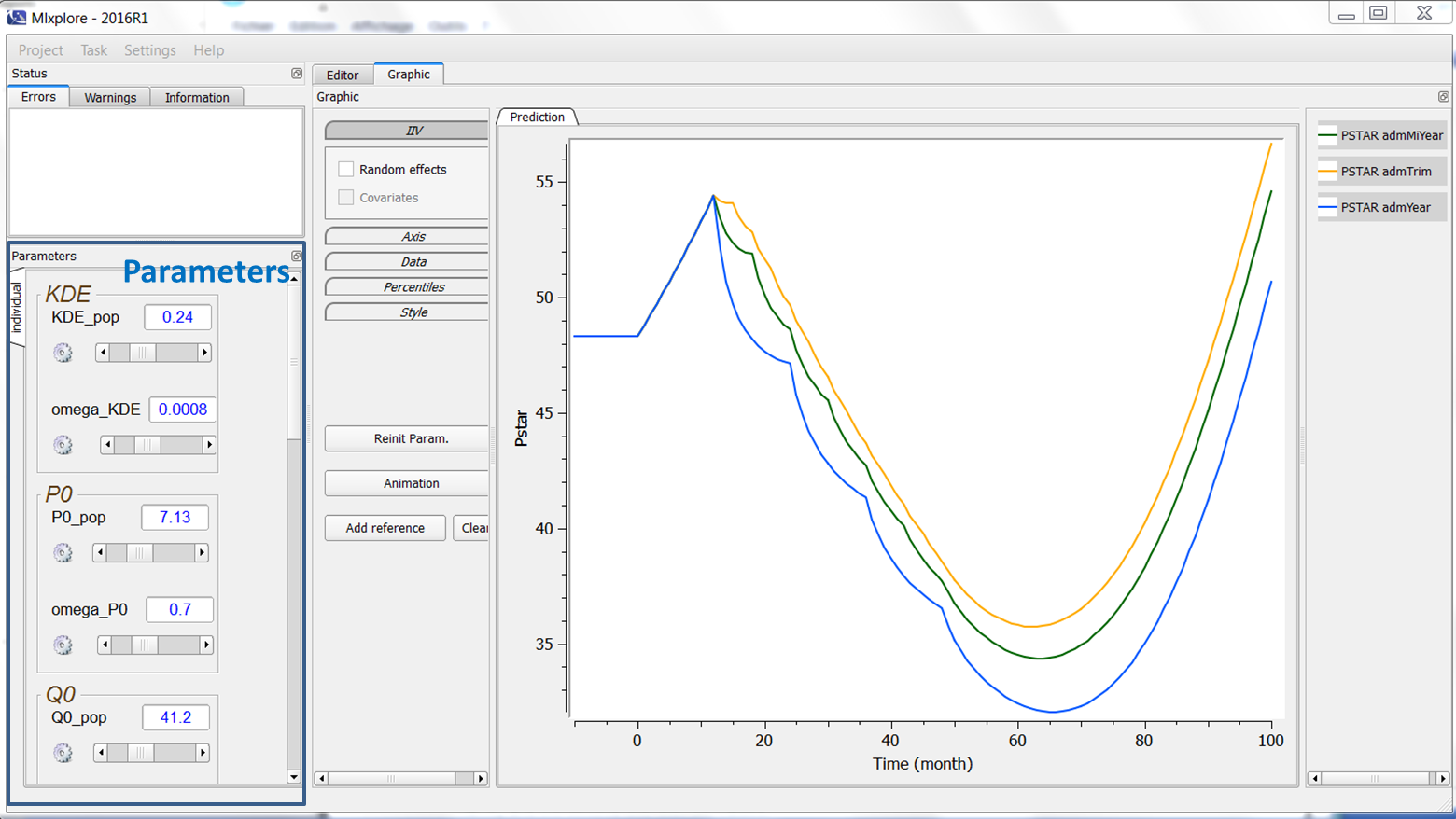
3.2.Parameters
Introduction
On the left of the interface, we can play with the parameters values. They are represented by their name, their value and a slider as can be seen on the following figure.
What can we do with the parameters?
One can play with the parameters in several ways :
- modify the value by typing a number directly in the numerical box.
- modify the value with the slider. By default, the bounds are half and twice the initial condition of the parameter. This can be modified by clicking on the button on the left where you can define manually the min and the max.
Why is there several parameters windows?
There are several windows corresponding to the several subsections of the model
- “prediction” corresponds to the inputs of the [LONGITUDINAL] subsection. Notice that Mlxplore does not take the error model into account, therefore, only the prediction is used. Thus, if an error model is defined, the slider for the parameter may appear but will have no impact on the prediction results.
- “individual” corresponds to the inputs of the [INDIVIDUAL] subsection. Notice that, when a distribution is defined for a parameter, all the parameters used to define the prediction are displayed in a common box. Moreover, if the distribution is defined with covariates and coefficients, the coefficients are included in the same box.
- “covariate” corresponds to the inputs of the [COVARIATE] subsection. It works exactly as the window individual.
Why are we abusively talking about real time?
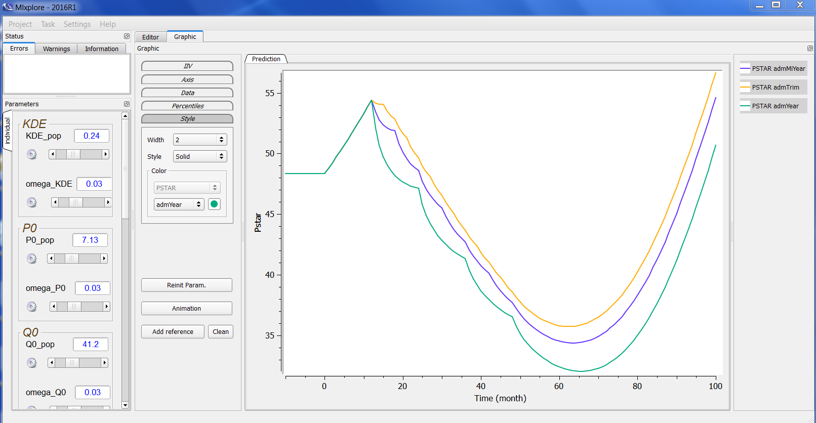
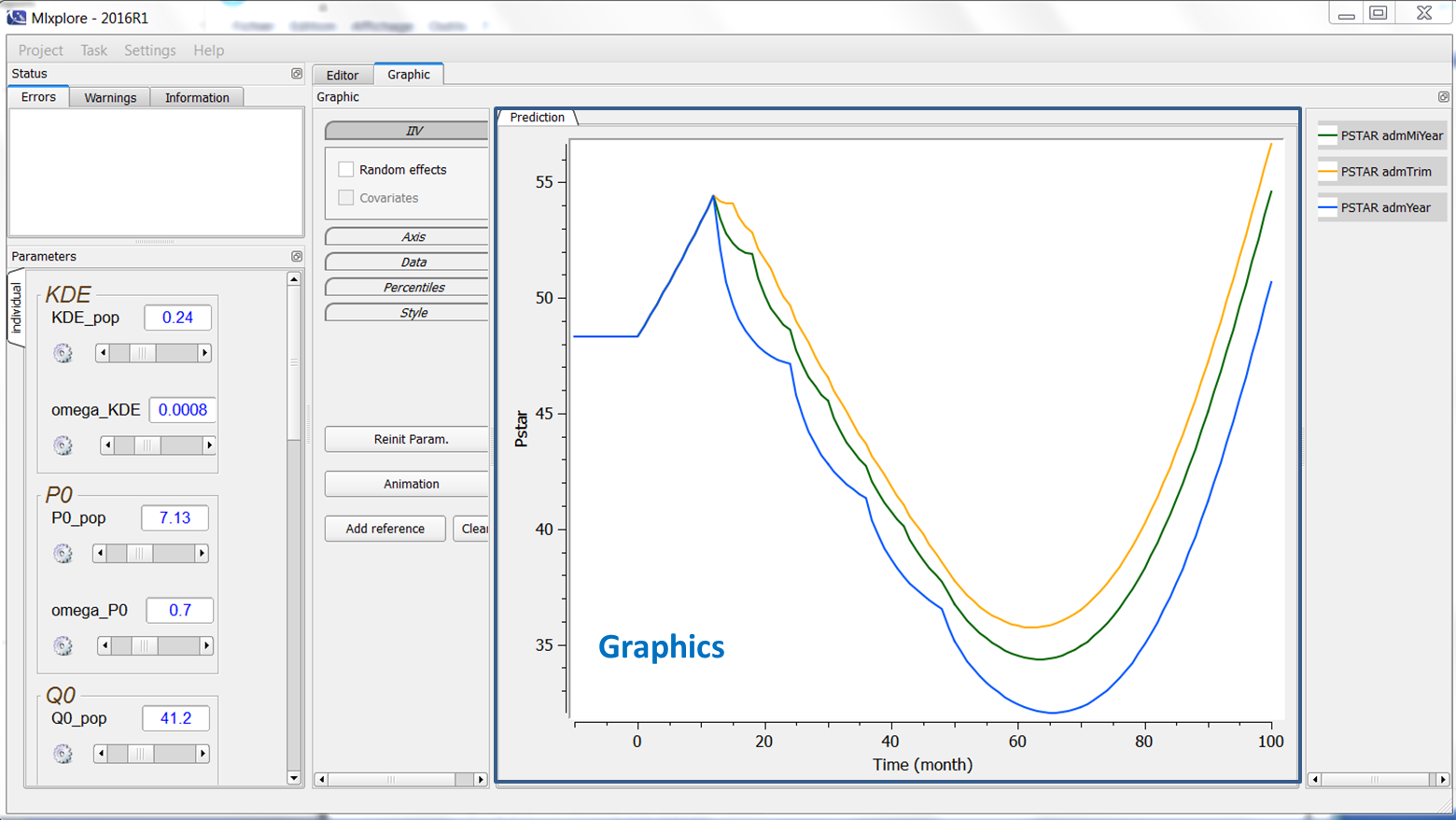
When the user modifies a parameter, the computation is instantaneously remade. The user sees directly the results in the graphics frame. For example, when modifying the parameter gamma_pop from 0.729 to .25, a new simulation is run and the graphic is updated as follows:
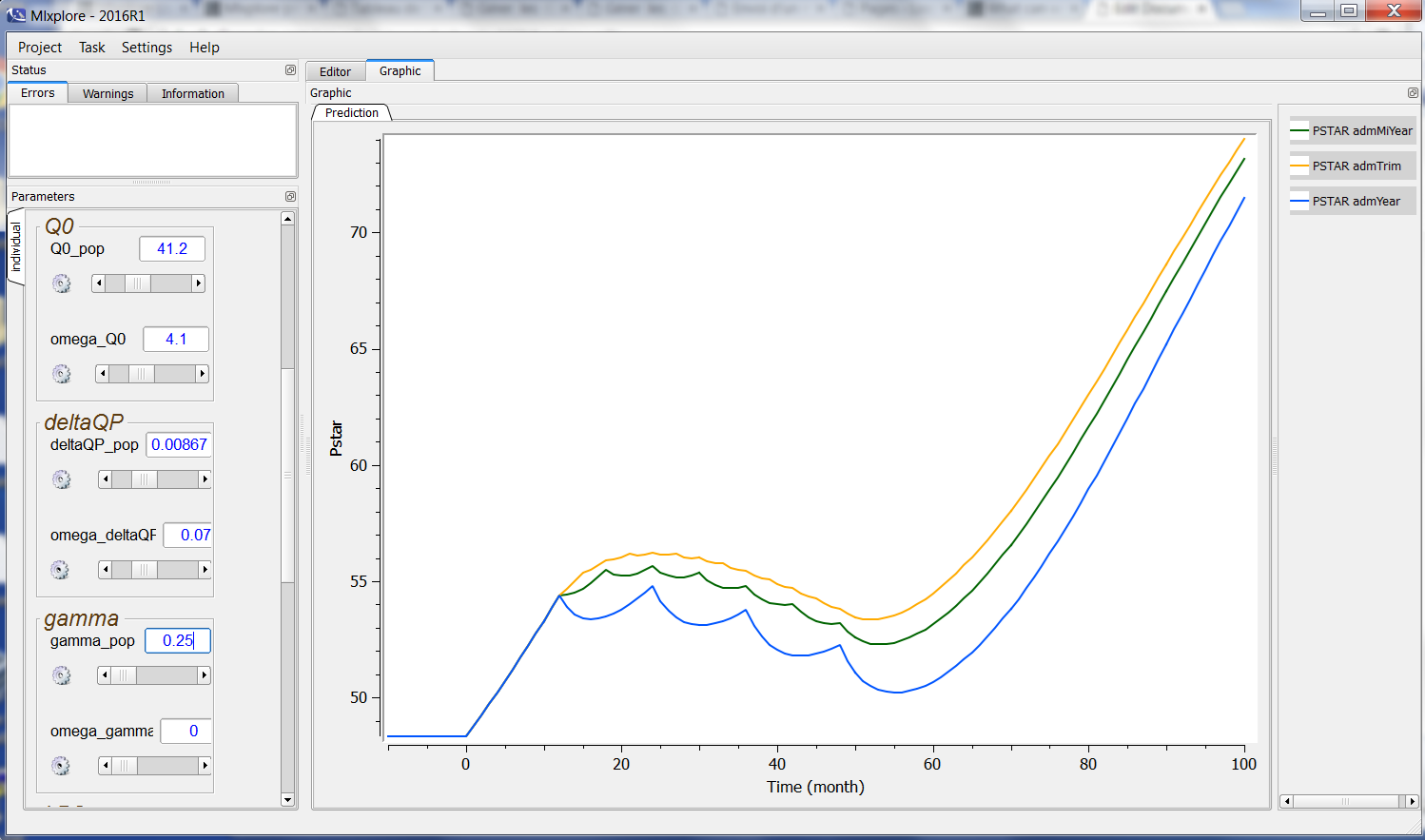
We abusively talk about real time. We do not have any pretension to be real-time. This is just to point out that the computations are fast and made automatically.
3.3.Graphics
Introduction
The graphics are the core of the interface. This window can be split in three parts: the graphics themselves, the associated legend, and the settings.
Graphics and legends
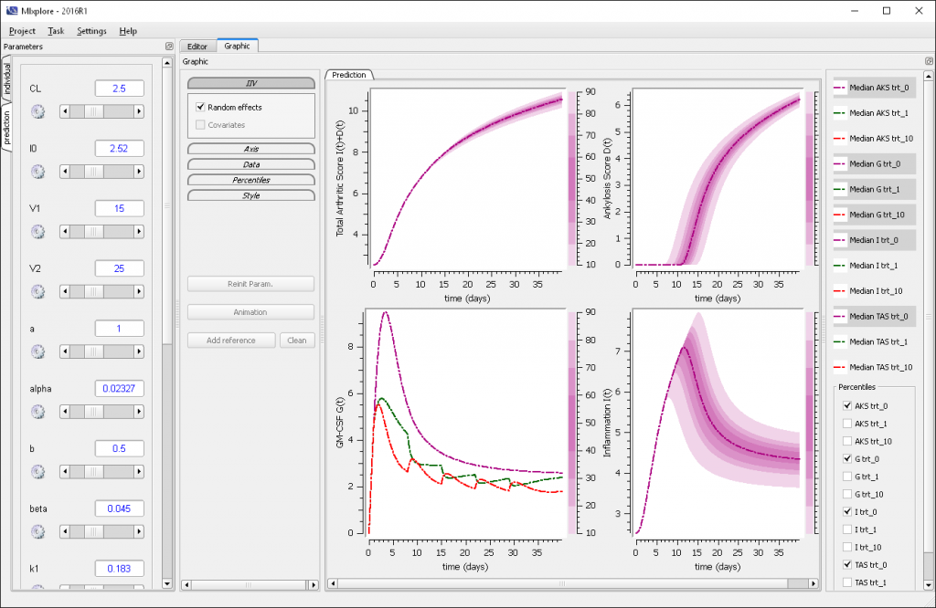
The graphics are displayed in the main window as can be seen in the following figure:
The legend of each prediction for each treatment is displayed on the right of the graphics. The name in the legend corresponds to the prediction name associated with the administration or treatment name. If no administration is done, the name is only the prediction name. All the elements of the graphics can be tuned using the graphics settings as follows.
Graphic settings
IIV
The user can activate and deactivate the display of inter-individual variability due to random effects and/or to covariates.
- If the “random effects” tick box is checked, individual parameters are drawn from the parameters distributions and 200 (by default) simulations are run.
- If the “covariates” tick box is checked, covariates are drawn from their distributions and used together with the population parameters to generate 200 individual parameters and run the corresponding simulations.
- If both boxes are ticked, individual parameters are drawn from the population distribution, taking into account the covariates drawn from their distributions.
Note that the check boxes for random effects and covariates are only available if the subsections [INDIVIDUAL] and [COVARIATE] exist.
Axis
For each plot, the user can choose
- The label of the X-axis, the possibility to display it in a log-scale and the variable for the X-axis. By default, the X-axis corresponds to the time, but one can look at an output w.r.t. another one for instance.
- The label of the Y-axis, the possibility to display it in a log-scale and the variables for the Y-axis. The user can choose the variables to display among all the outputs he has defined in the project. In addition, several outputs can be displayed on the same graphic.
- The limits of the X-axis and Y-axis. To set the limits manually, the user can click on “Manual limits” and choose the minimum and maximum values of the X-axis and the Y-axis. The maximum value must be strictly greater that the minimum value. To set the limits automatically, the user can click on “Auto limits”. By default, each graphic is set independently and automatically to its best values. The user can click on “Same X” and “Same Y” check boxes to share the same X-axis and Y-axis limits respectively.
Notice that when both iiv and log-scale for the Y-axis are activated, the graphic represents the log of the percentile of the variable of interest and not to the percentiles of the log of the variable of interest.
Data
The user can overlay data on the graphics. This is helpful in the pre-analysis to see if the model is representative of the data under consideration. In case of data with several individuals, all individuals are plotted with the same color. To see how to overlay data, click here.
Percentiles
In this tab, the user can define:
- Bands: The number of bands considered for the plot. By default, the value is 8. The value is bounded between 0 and 100.
- Level: The level under consideration. This means that the displayed percentile bands will go from
to
. By default, the value is 90, and it is bounded between 0 and 100.
- Simulations: The number of simulations performed. By default, the value is 200, and it is bounded between 1 and 10000.
 to
to  . By default, the value is 90, and it is bounded between 0 and 100.
Style
The user can define the style of all outputs. In terms of style, the line width and style (solid line, dashed line, etc) are common to all outputs. On the contrary, the color of each treatment for each variable can be defined by the user. By default, Mlxplore keeps the same colors as defined during the previous use.
Buttons
Several buttons are at the disposal of the user:
- “Reinit Param.” allows to reinitialize the parameters to the ones defined in the project file.
- “Animation” allows to make an animation of the predictions w.r.t. time. This is useful when an output is represented w.r.t. another one (rather than w.r.t. time).
- “Add reference” allows to freeze the currently displayed predictions. When moving the sliders, a second curve will appear. This is particularly useful when the user wants to compare predictions with varying parameters. For example, it is possible to add several references (named ref 1, ref 2, …) for several values of a parameter to see the impact of this parameter on the outputs. Notice that it is only possible to make references on the predictions, it is not possible to make references for the iiv simulation distributions.
- “Clean” cleans the references.
Notice that all the buttons are disabled when iiv are activated.
Legend
The legend is clickable to hide/unhide elements:
- clicking/unclicking on the prediction in the legend zone allows to hide/unhide the associated curve
- checking/unchecking the check box in the percentiles box allows to hide/unhide the associated distributions
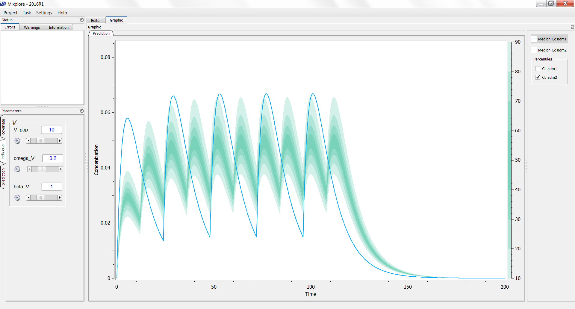
On the following example, we compare the same model with two different treatments. Using the legend, we can see the prediction of the first treatment (adm1 in blue) and the estimation of the variability of the second one (adm2 in green).
3.4.Adding a data set in the graphics
Introduction
It is possible to overlay a data set on the graphics using the “Browse” button in the “Data” frame.
Loading a data set
Firstly, it is possible to load a data set. By clicking on “Browse” and choosing a data set, a window appears. The user has to define which column is the time, which one is the measurements and which one is the YTYPE (if necessary).
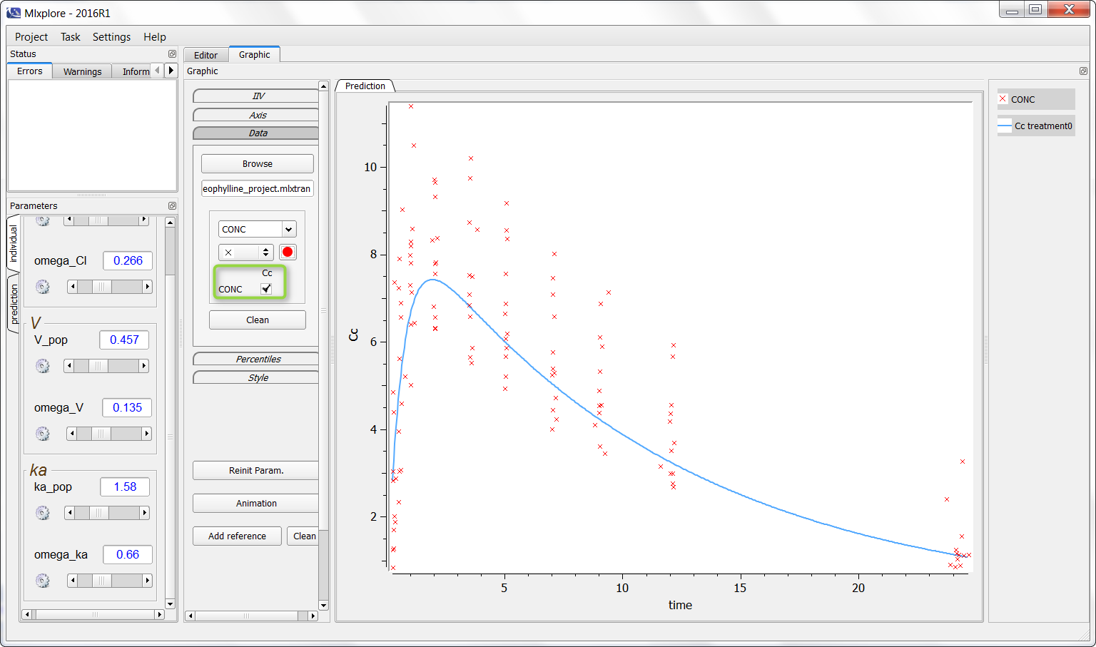
On the following example, a PK model was used and we would like to add the theophylline data set. One can click on “Browse” and choose the data as following (in the green box):
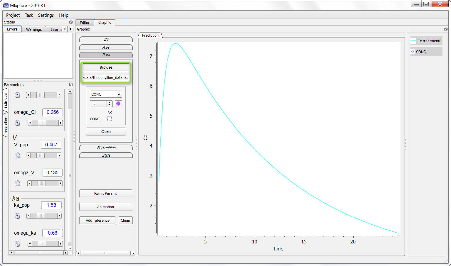
It is now possible to click (as in the green box) to overlay the data on the graphic as following:
Finally, one can activate the iiv simulations to see the representativity of the model with regards to the data set as on the following figure:
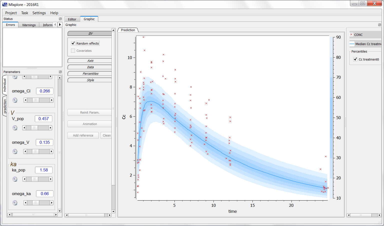
Notice that Mlxplore does not manage error models. Thus, the comparison between the model and the data set is not fully representative of the variability of the model.
Export function from Monolix
When exporting a project from Monolix to Mlxplore, the data set is directly loaded (but not displayed by default) and the parameters taken into account are those from Monolix interface.
3.5.Editors
Introduction
While modifications of the parameter values are done directly via the sliders in the interface, modifications of other project or model characteristics, such as the dose administration schedule for instance, are done via the editors.
Editor
The editor can be seen on the following figure: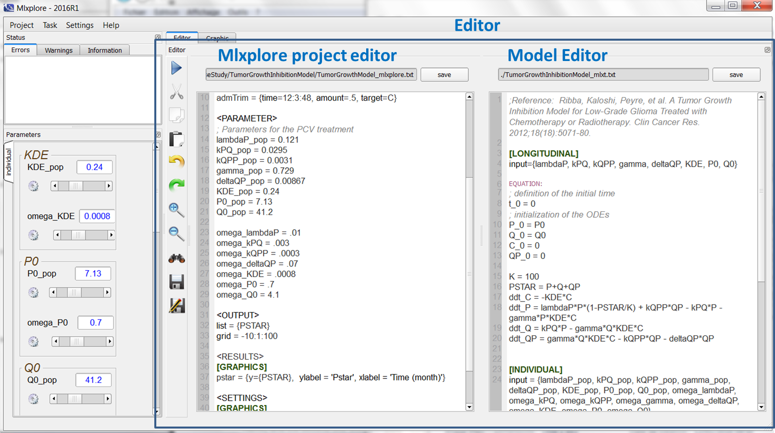
In the presented case, one uses two editors, one on the left that edits the Mlxplore project, and one on the right that describes the model. To run the model, the user just has to click on the arrow on the left.
Status window
When running the Mlxplore project, possible compilation errors or warnings are displayed in this windows. It allows the user to understand what is wrong and/or can be improved in his model definition. When the simulation results into NaNs, it is displayed in the warning window. The status window can be seen on the following figure:
4.FAQ
Parameters / Prediction
- If I move the error models parameters in the interface, nothing changes. Why? This is normal. Mlxplore does not manage error models as Mlxplore focuses on predictions. Thus, if an error model is defined, the slider for the parameter can appear but will have no impact on the prediction results.
Graphics / Axis
- When I check the log y axes, an error window pops us and the axis labels of the figure are not displayed correctly. I get all zeros instead of 10^-1, 10^-2 etc. What’s going on? Read the answer here.
Graphics / IIV
- When I activate the iiv, the graphics do not display all times. Why? When the iiv is activated, draws for the covariates and/or the individual parameters are done. This can load to NaN values in the simulations for some time points. Check the warnings in the status windows. To avoid the problem, you can add saturations for example before power calculation, logarithm calculation, …
- When I check the covariate/random effect tickbox in the iiv, nothing happens. Why? When the iiv is activated (for either the individual parameters and/or the covariates), samples from the associated distribution are used. If no distribution is defined, all simulations are done with the same (population) parameters, and lead to the same prediction. This is for instance the case for covariates iiv when you export a project from Monolix. For simulation purpose in Mlxplore, the exported project takes the mean value of the covariate of the data set and set this value for Mlxplore (unique value without a distribution). You can edit your model file via the editor to add a distribution for the covariates.
Project loading
- I get an error “Load file … error” while loading a project. What can I do? If in the “Errors” tab of Mlxplore, the error is “Parse not ended”, check if your dataset file contains only allowed characters.
- I get an error “Cannot load project : parse errors” while opening Mlxplore form Monolix. What can I do? The error may be due to unallowed characters in your dataset file. Check allowed characters here.
Running a project
- I get an error “Running model error !” while running a loaded project. If in the “Errors” tab of Mlxplore, the error is “Parse not ended”, check if your dataset file contains only allowed characters.
4.1.Work around on the log-scale
When I check the log y axes, then a error window pops us and the axis labels of the figure are no displayed correctly. I get all zeros instead of 10^-1, 10^-2 etc. What’s going on?
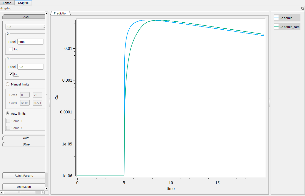
This is typically the case in the following example. In singledose.mlxplore.mlxtran (in the demo files in Userguide/2_TreatmentDesign/), a PK model is explored using two different treatments. Both treatments start at t=5. The following figure shows the results of the concentration for both treatments.
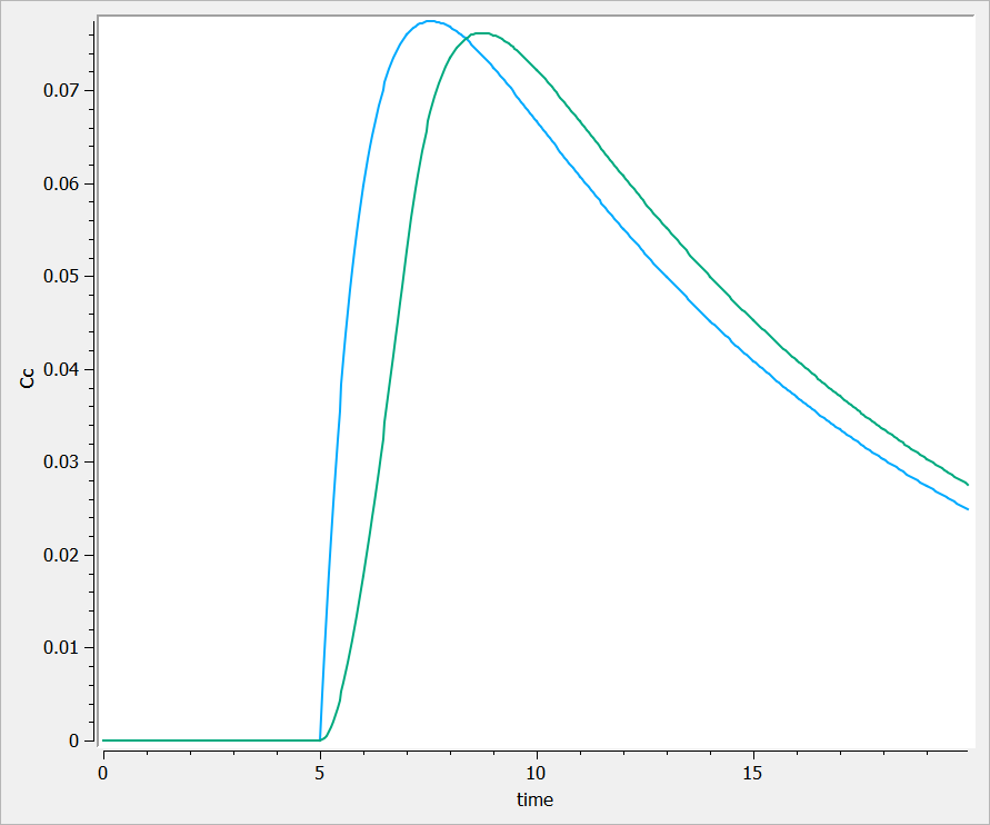
One can see that before t=5, both concentrations are equal to 0.
Clicking on log-scale for the Y-axis.
When clicking on the log-scale for the Y-axis, the following windows pops up explaining that there is an issue in the computation.
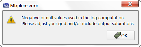
Thus, the proposed graphic provides a poor representation and the axes are not displayed correctly.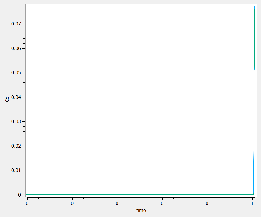
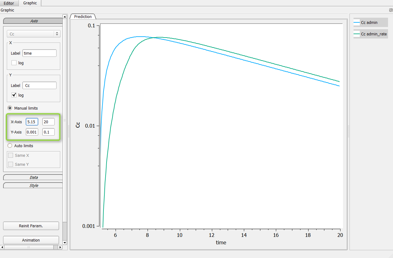
Possibility n°1: Change manually the axis
The first possibility is to change manually the axis of your graphic. For that, go in the axis setting, click on “Manual settings” as on the following figure (in the green box). In the presented case, one can set the minimum of the X-axis bigger than 5, and the Y-axis between .001 and .1 for example.
Possibility n°2: Change the grid in the Mlxplore project
It is possible to change it the grid in the project file via the editor and start it after 5 for example. In the following case, we set
grid = 5.05:.05:20
It leads to the following figure when clicking on the log-scale.

Possibility n°3: Add a saturation on your output
On the longitudinal model, the user can add a saturation function to make sure the concentrations are greater than a strictly positive value. In the following case, we set
Cc = max(Ac/V, 1e-6)
in the model file. It leads to the following figure when clicking on the log-scale.