Mlxplore Case Studies

1.Case studies #

Different cases studies are presented here to show how to use Mlxtran to define a model and how to use Mlxplore for model exploration.

Tumor growth model:

Tumor growth inhibition model exploration: The purpose of this example is the exploration of a tumor growth inhibition model for low-grade glioma treated with chemotherapy or radiotherapy. The model comes from a paper from Ribba et al. in Clinical Cancer Research (18(18); 5071–80). The research goal is to describe tumor size evolution in patients treated with chemotherapy or radiotherapy and to explore the impact of treatments on the tumor growth, along with the impact of inter-individual variability.

Delay modeling:

Using delays, the example of rheumatoid arthritis: Rheumatoid arthritis (RA) is an immune-mediated inflammatory disease and is characterized by a chronic inflammation and synovial hyperplasia leading to the destruction of cartilage and bone. Approximately one percent of the world-wide population suffers from RA. The model comes from a poster published at PAGE in 2011 by Gilbert Koch. The research goal is to develop a multi response model to describe the time course of the total arthritic score and the strongly delayed ankylosis score measured in collagen induced arthritic (CIA) mice. The authors used a three compartment delay differential equation model to get a deeper understanding between cytokine level, inflammation and bone destruction.

Pharmacokinetic modeling:

Tobramycin pharmacokinetics: In this example, the pharmacokinetics of Tobramycin, an antimicrobial agent, is explored. It is part of a case study crossing over all applications (Datxplore, Monolix, Mlxplore, Simulx).

Physiologically-based pharmacokinetic (PBPK) models:

Glucose-insulin model: the example explores the homeostasis of glucose and insulin plasma concentrations after glucose or carbohydrate uptakes as performed during glucose tolerance tests. The PBPK model represents glucose, insulin, incretins and glucagon and has 28 equations.

Target-mediated drug disposition models:

TMDD models: TMDD models exhibit a characteristic concentration-time profile. Each parameter of the model has a precise impact that we can visualize using Mlxplore. This knowledge helps to determine which parameter are identifiable depending on the data set.

Treatment explorations:

From single dose to multiple doses: after having estimated a PK model on a single dose data set, the model is exported to Mlxplore to explore new dosing regimens, in particular multiple doses. The simulations are overlaid with actual data for comparison.

To see all the case studies in a single page and/or export it as a pdf? Please go to this page.

2.Tumor growth inhibition model exploration #

Introduction

The purpose of this case study is the exploration of a tumor growth inhibition model for low-grade glioma treated with chemotherapy or radiotherapy. The model has been published in Ribba et al. in Clinical Cancer Research (18(18); 5071–80). The research goal is to describe the tumor size evolution in patients treated with chemotherapy or radiotherapy, and to explore the impact of treatments on the tumor growth, along with the impact of inter-individual variability.

Tumor growth inhibition model

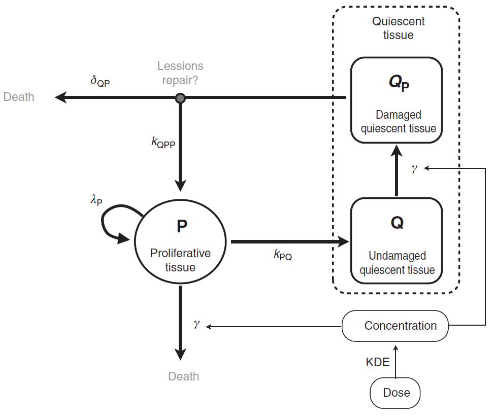
The tumor is composed of proliferative (P) and nonproliferative quiescent tissue (Q), expressed in millimeters. The transition of proliferative tissue into quiescence is governed by a rate constant denoted $k_{PQ}$ . The treatment directly eliminates proliferative cells by inducing lethal DNA damage while cells progress through the cell cycle. The quiescent cells are also affected by the treatment and become damaged quiescent cells ( $Q_{P}$ ). Damaged quiescent cells, when re-entering the cell cycle, can repair their DNA and become proliferative once again (transition from $Q_{P}$ to P) or can die because of unrepaired damages.
The pharmacokinetics of the PCV chemotherapy is modeled using a PK/PD approach, in which drug concentration is assumed to decay according to an exponential function. In this model, the three administrated drugs were not considered separately. Rather, the authors assumed the treatment to be represented as a whole by a unique variable (C), which represents the concentration of a virtual drug encompassing the 3 chemotherapeutic components of the PCV regimen. Following Ribba et al., the model writes

$\left\{\begin{array}{l}\frac{dC}{dt} = - KDE \times C \\\frac{dP}{dt} = \lambda_{p}P(1-\frac{P^{\star}}{K})+k_{Q_{P}P}\times Q_{P}-k_{PQ}\times Q - \gamma_{P} KDE \times C \times P\\\frac{dQ}{dt} = k_{PQ}P-\gamma_Q \times C \times KDE \times Q \\\frac{dQ_{P}}{dt} = \gamma_{Q}\times C \times KDE \times Q - k_{Q_{P}P}Q_{P}-\delta_{QP}\times Q_{P}\\P^{\star} = P+Q+Q_{P}\end{array}\right.$

Notice that, in the publication, $\gamma_P=\gamma_Q=\gamma$ was assumed for identifiability reasons. The initial condition writes

$\left\{\begin{array}{l}C(t=0) = 0 \\P(t=0) = P_{0}\\Q(t=0) = Q_{0}\\Q_{P}(t=0) = 0\end{array}\right.$

A schematic view of the model proposed in Ribba et al. is represented here:

TumorGrowth_ModelSchematicView

How to model it in Mlxtran

The purpose here is to define the model in Mlxtran language. The model writes as 4 ODEs. The resulting set of parameters is $(\lambda_P, k_{PQ}, k_{Q_{P}P}, \delta_{Q_{P}}, \gamma, {\rm KDE})$ , with 2 initial conditions, $(P_{0}, Q_{0})$ . Therefore, the [LONGITUDINAL] subsection starts with

[LONGITUDINAL] 
input={lambdaP, kPQ, kQPP, gamma, deltaQP, KDE, P0, Q0}

Then, we start the EQUATION: block with the initial conditions:

EQUATION:
; definition of the initial time
t_0 = 0
; initialization of the ODEs
P_0 = P0
Q_0 = Q0
C_0 = 0
QP_0 = 0

and continue it with the 4 ODEs and the definition of $P^{\star}$

K = 100
PSTAR = P+Q+QP
ddt_C = -KDE*C
ddt_P = lambdaP*P*(1-PSTAR/K) + kQPP*QP - kPQ*P - gamma*P*KDE*C
ddt_Q = kPQ*P - gamma*Q*KDE*C
ddt_QP = gamma*Q*KDE*C - kQPP*QP - deltaQP*QP

The individual parameters corresponding to the 8 population parameters (6 parameters and 2 initial conditions) were assumed to be log normally distributed across individuals. Therefore, we have to define an [INDIVIDUAL] subsection as follows:

[INDIVIDUAL]
input = {lambdaP_pop, kPQ_pop, kQPP_pop, gamma_pop, deltaQP_pop, KDE_pop, P0_pop, Q0_pop, 
omega_lambdaP, omega_kPQ, omega_kQPP, omega_deltaQP, omega_KDE, omega_P0, omega_Q0}  

DEFINITION:
lambdaP = {distribution = lognormal, typical = lambdaP_pop, sd = omega_lambdaP}
kPQ     = {distribution = lognormal, typical = kPQ_pop,     sd = omega_kPQ}
kQPP    = {distribution = lognormal, typical = kQPP_pop,    sd = omega_kQPP}
gamma   = {distribution = lognormal, typical = gamma_pop,   sd = omega_gamma}
deltaQP = {distribution = lognormal, typical = deltaQP_pop, sd = omega_deltaQP}
KDE     = {distribution = lognormal, typical = KDE_pop,     sd = omega_KDE}
P0  = {distribution = lognormal, typical = P0_pop,          sd = omega_P0}
Q0  = {distribution = lognormal, typical = Q0_pop,          sd = omega_Q0}

The model is then the sum of all these codes and is implemented in TumorGrowthInhibitionModel_mlxt.txt

Model and treatment exploration: project definition

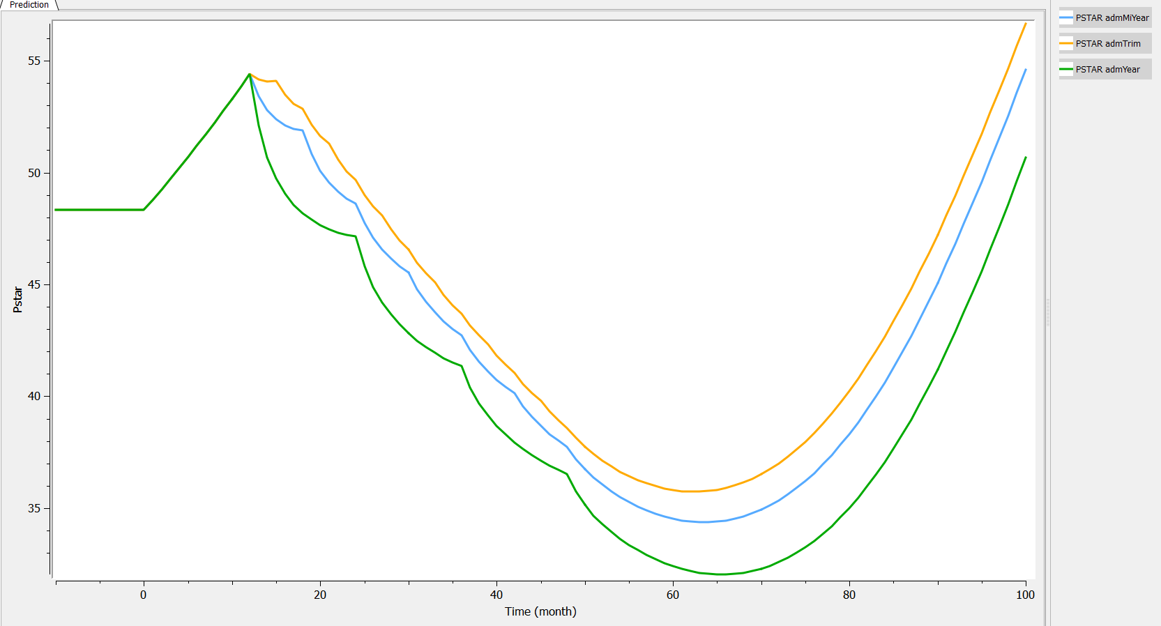
To define the project, we must define the model (in the <MODEL> section, as done in the previous paragraph), all parameter values (for the *_pop and omega_*, in the <PARAMETER> section) and the output (name and time grid, in the <OUTPUT> section). To explore the model, we define in the section <DESIGN> three administrations where we vary the inter dose timing and keep the same annual amount.

“admYear”, where we administrate an amount of 2 each 12 months starting after 12 months
“admMiYear”, where we administrate an amount of 1 each 6 months starting after 12 months
“admTri”, where we administrate an amount of .5 each 3 months starting after 12 months

Finally, a section is added to define the graphic we want to look at. Then, the project is implemented in TumorGrowthModel_mlxplore.txt as follows:

<MODEL>
file = './TumorGrowthInhibitionModel_mlxt.txt'

<DESIGN>
[ADMINISTRATION]
admYear = {time=12:12:48, amount=2, target=C}
admMiYear = {time=12:6:48, amount=1, target=C}
admTrim = {time=12:3:48, amount=.5, target=C}

<PARAMETER>
; Parameters for the PCV treatment
lambdaP_pop = 0.121
kPQ_pop = 0.0295
kQPP_pop = 0.0031
gamma_pop = 0.729
deltaQP_pop = 0.00867
KDE_pop = 0.24
P0_pop = 7.13
Q0_pop = 41.2

omega_lambdaP = .03
omega_kPQ = .03 
omega_kQPP = .03 
omega_deltaQP = .03 
omega_KDE = .03 
omega_P0 = .03
omega_Q0 = .03 

<OUTPUT>
list = {PSTAR}
grid = -10:1:100

<RESULTS>
[GRAPHICS]
pstar = {y={PSTAR},  ylabel = 'Pstar', xlabel = 'Time (month)'}

Model exploration: graphical results

Two aspects can be analyzed: the predictions and the inter-individual variability. First we can explore the predictions associated with the three kinds of administrations:

TumorGrowth_Prediction

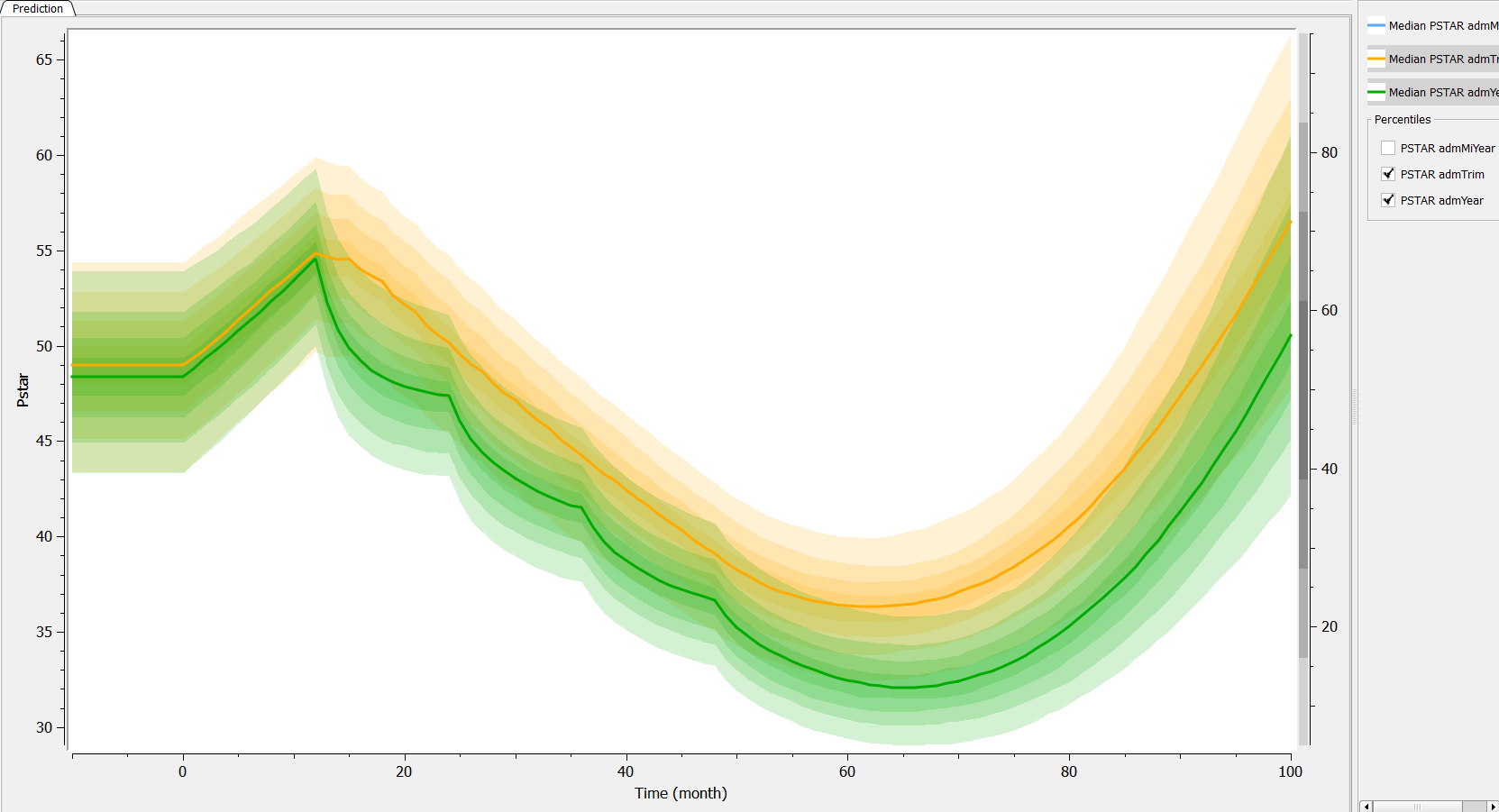
Then, if one wants to explore the impact on the inter-individual variability, one can click on iiv leading to the following figure:

TumorGrowth_iiv

Conclusion

In this example, a relatively complex ODE model has been implemented in Mlxtran, and its behavior (predictions following different treatments, as well as inter-individual variability) as been explored with Mlxplore.

3.Using delay in modeling, the example of rheumatoid arthritis #

Introduction

Rheumatoid arthritis (RA) is an immune-mediated inflammatory disease and is characterized by a chronic inflammation and synovial hyperplasia leading to the destruction of cartilage and bone. Approximately one percent of the world-wide population suffers from RA. The model is presented in a poster published at PAGE in 2011 by Gilbert Koch. The research goal is to develop a multi response model to describe the time course of the total arthritic score and the strongly delayed ankylosis score measured in collagen induced arthritic (CIA) mice. The authors used a three compartment delay differential equation model to get a deeper understanding between cytokine level, inflammation and bone destruction.

A multi-response model for rheumatoid arthritis

The modeling part was done in three steps. We will follow the steps presented by Koch in his PhD thesis.

Modeling Step 1: The cytokine behavior in time.
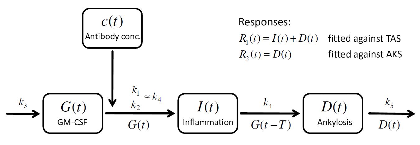
The cytokine GM-CSF (noted $G$ ) drives the disease. Its kinetics is described by:

$\frac{dG}{dt} = k_3-\frac{k_1}{k_2}(1-e^{-k_2t})G(t) - E(Cc(t))G(t)$

The last term models the effect (function $E$ ) of the anti-GM-CSF antibody concentration ( $Cc$ ) on the cytokine GM-CSF level $G$ . The effect of the antibody is described by the following expression: $E(Cc)=(\sigma_1*\exp(- \sigma_2*Cc) + \sigma_3)*Cc$ .

The concentration of the anti-body is described by a 2 compartment model with bolus administration and linear elimination.

Modeling Step 2: Multi-response approach to model the TAS and AKS
The mathematical model of the arthritic disease is split into an inflammatory part $I(t)$ and an ankylosis (bone and cartialge destruction) part $D(t)$ and the sum $R_1(t) = I(t) + D(t)$ defines the response $R_1(t)$ , which corresponds to the experimentally measured total arthritic score (TAS). In addition a second response function is defined as $R_2(t) = D(t)$ which corresponds to the ankylosis score (AKS).
To build a model for the time course of the inflammation $I(t)$ and the ankylosis $D(t)$ , the concept of lifespan modeling is introduced: the overall inflammation $I(t)$ is controlled by two processes, the inflow $k_{in}(t)$ and the outflow $k_{out}(t)$ . Assuming that the inflammation caused by these processes remains a certain time period $\tau$ and is driven by the amount of GM-CSF, one obtains $k_{out}(t) = k_{in}(t-\tau)$ and $k_{in}(t) = k_4 G(t)$ where $k_4$ is a first order rate constant. Then the total balance equation for the inflammation reads:

$\frac{dI}{dt} (t) = k_4G(t) - k_4G(t - \tau)$

Similarly, for the ankylosis $D(t)$ one obtains $k_{in}(\textrm{ankyloses}) = k_{out}(\textrm{inflammation})$ . Applying a first order loss term $k_{out}(\textrm{ankyloses}) = k_5D(t)$ leads to the equation:

$\frac{dD}{dt} (t) = k_4G(t-\tau) - k_5G(t)$

The presence of $G(t)$ and $G(t - \tau)$ reflects that the inflammation and the ankylosis are driven by GM-CSF. Moreover, the action of GM-CSF on the ankylosis is delayed by $\tau$ . A schematic view of the model, proposed in Koch’s PhD thesis, is given here:

ArthritisSchematic

How to model it in Mlxtran

The purpose here is to define the model in Mlxtran language. The system writes as a PKPD model with a DDE. The resulting set of parameters is (alpha, beta, CL, V1, V2) for the PK model, (sigma1, sigma2, sigma3) for the effect model, and (k1, k2, k3, k4, k5, tau) for the RA model along with 3 additional initial conditions (I0, a,b). Therefore, the [LONGITUDINAL] subsection starts with:

[LONGITUDINAL]
input = {a, b, I0, alpha, beta, CL, V1, V2, sigma1, sigma2, sigma3, k1, k2, k3, k4, k5, tau}

Then, we start the EQUATION: block with the initial conditions:

EQUATION:
; initialization of the time
t0 = 0

; initialization of the variables of interest
I_0 = I0
D_0 = 0
G_0 = a*exp(b*t)

Notice that the initialization of the variable G is not only at time 0 but also across the past $[-\tau, 0]$ . One continues with the PKPD model:

K12 = alpha*beta*V2/CL
K21 = alpha*beta*V1/CL
Cc = pkmodel(k12=K12,k21=K21,V=V1,Cl=CL)
E = (sigma1*exp(- sigma2*Cc) + sigma3)*Cc

and the ODE/DDE equations along with the definition of the TAS and the AKS:

ddt_G = k3 - E*G - (k1/k2)*(1- exp(- k2*t))*G
ddt_I = k4*G - k4*delay(G,tau)
ddt_D = - k5*D + k4*delay(G,tau)

TAS = I+D
AKS = D

Finally, the individual parameters representing the variability of the delay are defined as a normal distribution and one writes:

[INDIVIDUAL]
input = {tau_pop, omega_tau}

DEFINITION:
tau = {distribution = normal, mean = tau_pop, sd = omega_tau}

The model is then the sum of all this code and is implemented in arthritisModel_mlxt.txt

Model and treatment exploration: project definition

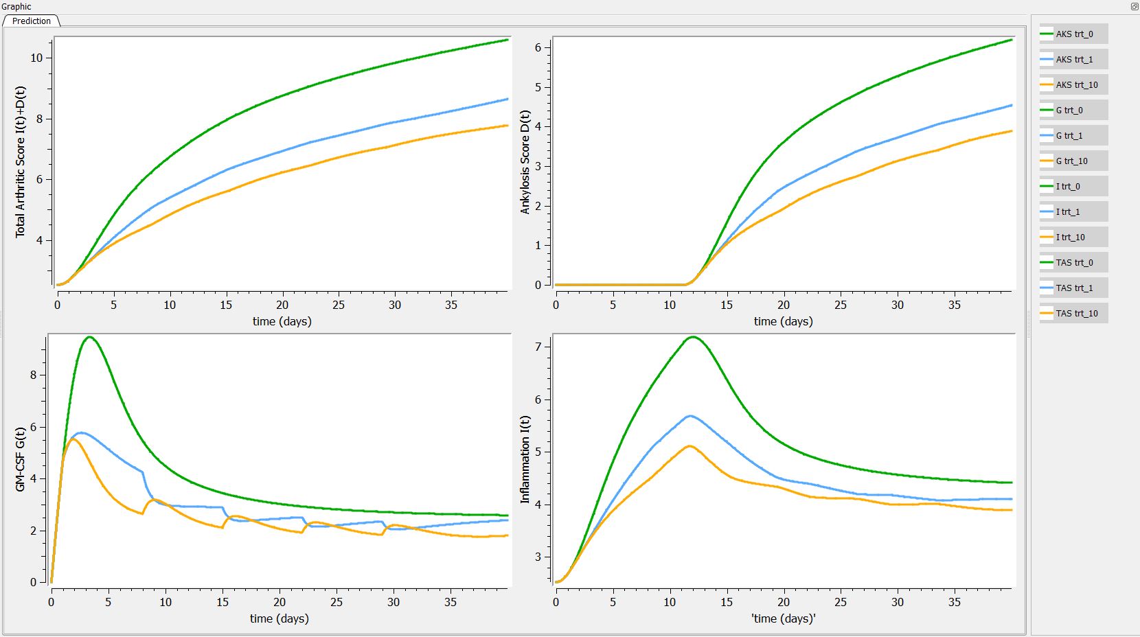
To define the project, one must define the model (done in the previous paragraph, section <MODEL>), the parameter values (section <PARAMETER>) and the output (section <OUTPUT>). To explore the model, we define in the section <DESIGN> three administrations where we vary the amount of antibody.

“Trt_0”, where we administrate nothing
“Trt_1”, where we administrate 1 mg/kg (and thus 70mg) each week during 5 weeks
“Trt_1”, where we administrate 10 mg/kg (and thus 700mg) each week during 5 weeks

Finally, a section is added to define the graphics we want to look at. The project is implemented in arthritisModel_mlxplore.txt as follows

;model definition
<MODEL>
file='./arthritisModel_mlxt.txt'

<DESIGN>
[ADMINISTRATION]
trt_0 = {time = {1, 8, 15, 22, 29}, amount = 0}
trt_1 = {time = {1, 8, 15, 22, 29}, amount = 70}
trt_10 = {time = {1, 8, 15, 22, 29}, amount = 700}

;parameter initial values
<PARAMETER>
; Initialization parameters
a = 1
b = 0.5
I0 = 2.52

; PK model 
alpha = 0.02327
beta = .045
CL = 2.5
V1 = 15
V2 = 25

; Effect model 
sigma1 = 0.154
sigma2 = 0.065
sigma3 = 0.003

; Arthritis model parameters
k1 = 0.183
k2 = 0.092
k3 = 5
k4 = 0.064
k5 = 0.016
tau_pop = 11.2
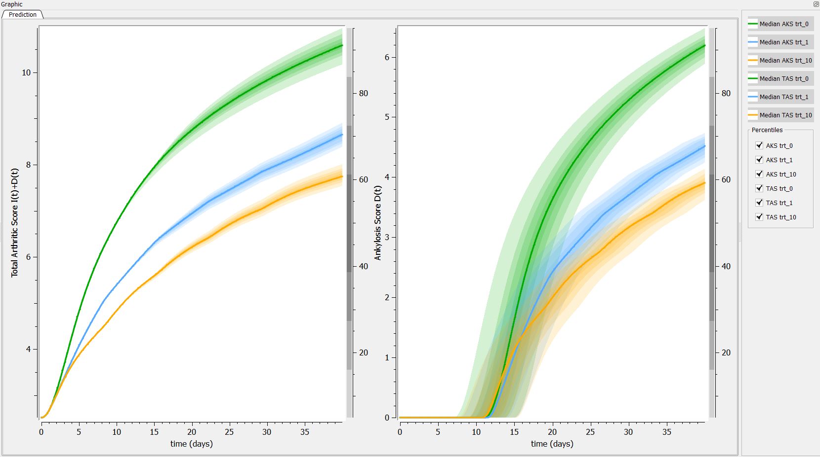
omega_tau = 3

;prediction outputs and grid
<OUTPUTS>
list={TAS,AKS, G, I, D,Cc}
grid=0:.01:40

<RESULTS>
[GRAPHICS]
pTAS = {y={TAS},  ylabel = 'Total Arthritic Score I(t)+D(t)', xlabel = 'time (days)'}
pAKS = {y={AKS},  ylabel = 'Ankylosis Score D(t)', xlabel = 'time (days)'}
pG = {y={G},  ylabel = 'GM-CSF G(t)', xlabel = 'time (days)'}
pI = {y={I},  ylabel = 'Inflammation I(t)', xlabel = 'time (days)'}
gridarrange(pTAS, pAKS, pG, pI, 2,2)

<SETTINGS>
[GRAPHICS]
nb_simulations = 200

Model exploration: graphical results

First we can explore the predictions following the 3 different treatments:

Arthritis
Then, if one want to explore the impact on the inter-individual variability on the delay, one can click on iiv leading to the following figure:

ArthritisDelay

Conclusion

In this example, we have implemented a model with ODEs, and DDEs with complex initial conditions using Mlxtran. Using Mlxplore, we have explored the influence of different treatments on the predictions. Mlxplore also enables to visualize the inter-individual variability.

4.Tobramycin case study - Part 4: Model exploration with Mlxplore #

Download data set only | Datxplore project files | Monolix project files | Mlxplore project files | Simulx scripts

This case study presents the modeling of the tobramycin pharmacokinetics, and the determination of a priori dosing regimens in patients with various degrees of renal function impairment. It takes advantage of the integrated use of Datxplore for data visualization, Mlxplore for model exploration, Monolix for parameter estimation and Simulx for simulations and best dosing regimen determination.

The case study is presented in 5 sequential parts, that we recommend to read in order:

Part 4: Model exploration with Mlxplore

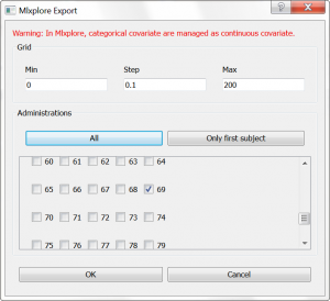
In this part, we would like to explore the influence of the parameters of a 2-compartment model. From the Monolix GUI, where we have selected a (V,k,k12,k21) model from the PK library, we have clicked on the blue icon to open Mlxplore. In the pop-up window, we can choose which individual we would like to simulate. We choose individual 69, which has only a few doses administrated, and modify the time grid to 0:0.1:200 as shown below:

CS-tobramycin-mlxplore-1-popup

In the Mlxplore application that has opened, a script has been automatically generated to define the simulation to run. The script contains information about:

the data file, to overlay the data on top of the simulation
the model, with its longitudinal part (structural model (V,k,k12,k21) from the library), the covariates, and the distributions for the individual parameters
the parameter values, taken from the Monolix GUI and the covariates taken from the data set
the administrations, with time and amount information, taken from the data set for individual 69
the output to display, and the time grid

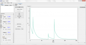
This script is editable, but let’s first run it as is, by clicking the blue arrow run button. The simulation is displayed. One sees the 4 administrations of different doses, and the non-linearity during the elimination phase. Using the sliders on the left, one can observe the influence of the parameter values on the simulation. Clicking the “Add reference” button permits to freeze a curve to better compare.

CS-tobramycin-mlxplore-2-fullGUI

As having several doses is not very convenient, we can go back to the editor tab and modify the [ADMINISTRATION] subsection to

adm1_1={ type=1,time={10}, amount={100} }

such that only one dose at time 10 and of amount 100 is administrated. We also modify the time grid to

grid=0:0.1:70

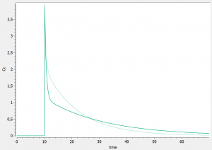
and run the model again. For instance, the influence of reducing the value of k21 (dark curve versus light curve) can well be understood:

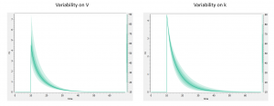
CS-tobramycin-mlxplore-3-k21impact

In addition to the individual parameters, the inter-individual variability (iiv) can also be visualized. In order to explore the impact of the iiv for each parameter individually, we first set all omega_* values to 0, except for the volume V. We then tick the “Random effects” box in the IIV tab. The prediction distribution is displayed, and one can see that the inter-individual variability on V will mainly influence the maximal level after the bolus dose. On the contrary, inter-individual variability on k has more impact at intermediate times after the dose:

CS-tobramycin-mlxplore-4-variability

One can also go to the “covariate” tab on the left, and play with the covariate values to see their impact on the simulation.

To change percentile levels, colors, labels, scales, etc look into the various menu tabs. To change the sliders limits, click on the sprocket.

With Mlxplore we have better understood the influence of the parameters, and the influence of the inter-individual variability.

Next part: Simulations for individualized dosing with Simulx and Monolix

5.PBPK glucose-insulin model exploration #

The purpose of this case study is to explore the homeostasis of glucose and insulin plasma concentrations after glucose or carbohydrate uptake.

Introduction

Disregulation of the glucose homeostasis is the cause of diabetes mellitus. To diagnose this disease, glucose and insulin monitoring after glucose uptake are performed during clinical tests, such as the oral glucose tolerance test (OGTT), the intravenous glucose tolerance test (IVGTT) and the mixed-meal glucose tolerance test (MGTT).

To simulate these clinical tests, a physiologically-based glucose-insulin model has been developed for healthy humans in:

Alvehag, K., & Martin, C. (2006, December). The feedback control of glucose: on the road to type II diabetes. In Decision and Control, 2006 45th IEEE Conference on (pp. 685-690). IEEE.

We use this model for this case study.

Physiologically-based glucose-insulin model

Plasma glucose levels are tightly regulated by the human body to ensure a constant delivery of this energy source to all tissues. After a meal, the increased glucose supply from the ingested food must be counterbalanced by an uptake of glucose by the liver for storage. On the opposite, during fast, the liver releases glucose. Glucose metabolism is tightly linked to insulin metabolism. Insulin is produced by the pancreatic cells when plasma glucose levels are high to promote glucose uptake by muscles and other organs. Other hormones are also involved in glucose homeostasis: incretins are released in the gut after glucose ingestion and stimulate insulin production. On the other hand, glucagon is produced when glucose levels are low and promotes the release of glucose from the liver.

To capture the human body physiology and the different sites of production and consumption of glucose and insulin a physiologically-based (PB) approach has been undertaken. In a PB model, the main organs are represented by well-stirred compartments connected via blood flow rates. This permits to easily model different kinds of perturbations as there is a close to 1-to-1 mapping between the human body parts and the model. Organ volumes and blood flow rates are well-known fro the human body, while parameters related to the metabolism in the various organs must be estimated from data or literature.

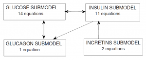
In the Alvehag et al. model, glucose and the three hormones (insulin, incretins and glucagon) were included as inter-connected submodels. The scheme below (from Alvehag et al.) summarizes the number of equations in each submodel and the submodel interconnections. In total, the model encompasses 28 equations, partly non-linear.

Glucose submodel

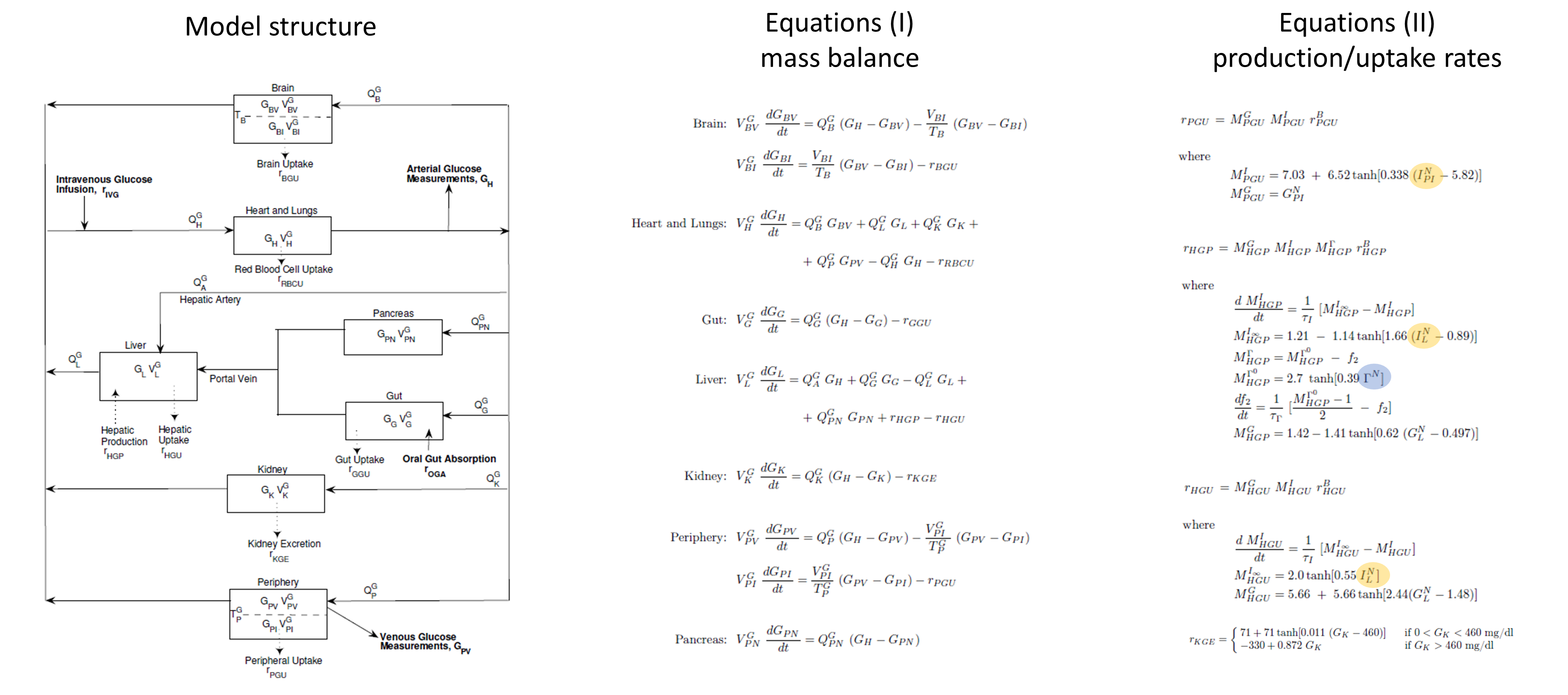
The glucose PB submodel is composed of the main organs involved in glucose metabolism: brain, pancreas, gut, liver, kidney, periphery (such as muscles) and heart and lungs. The scheme below (from Alvehag et al.) gives an overview of the model. The interconnection to the insulin submodel is highlighted in yellow and that to the glucagon model in blue. The details are given in Alvehag et al.

Insulin submodel

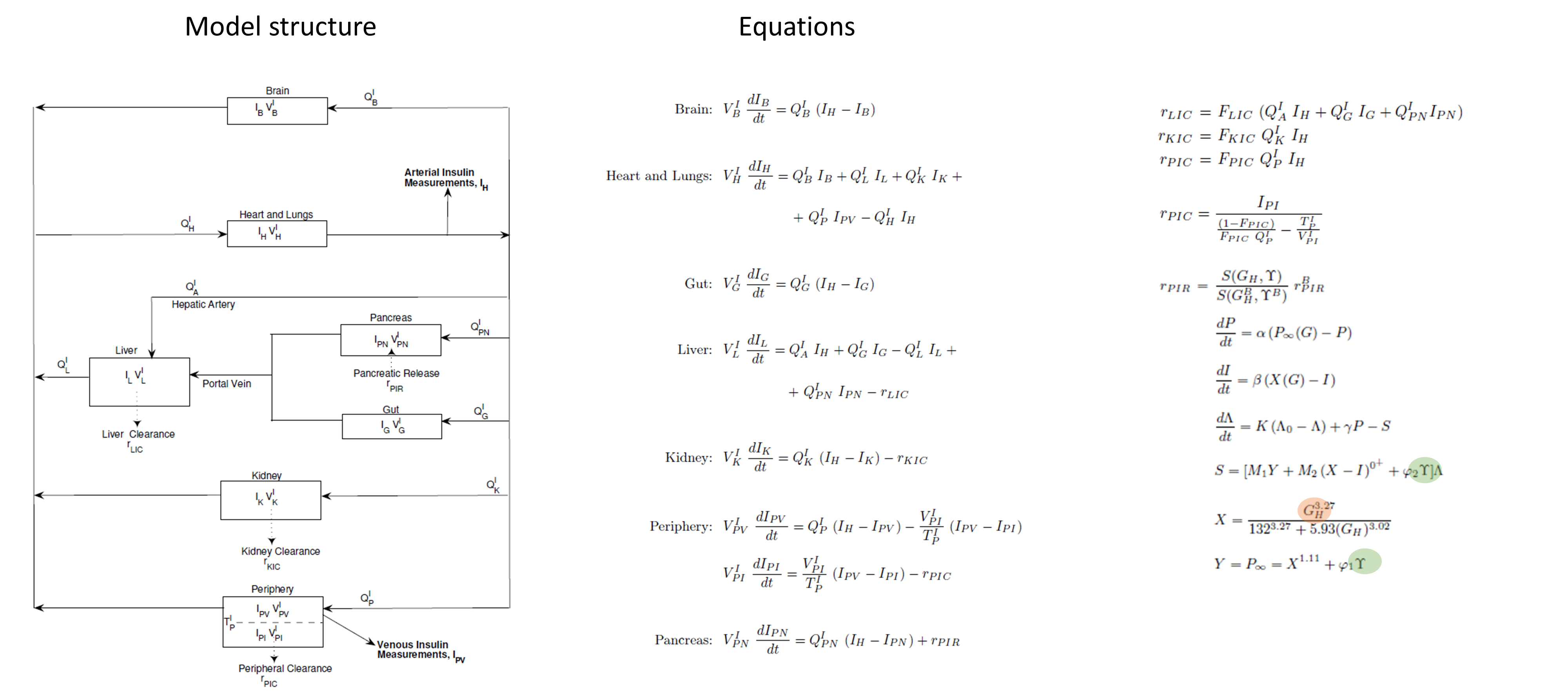
The insulin submodel is composed of the same organs as the glucose submodel. The scheme and equations are given below. The connection to the glucose model is in orange and to the incretins model in green.

Incretins and glucagon submodels

For glucagon and incretins only one compartment is considered, representing the entire body.

Glucose tolerance tests

The glucose tolerance tests are modeled in the following way:

intravenous glucose tolerance test (IVGTT): short infusion of glucose, applied directly to the venous glucose concentration
oral glucose tolerance test (OGTT): rapid first-order absorption with a transit compartment representing the stomach
mixed-meal glucose tolerance test (MGTT): slow first-order absorption with a transit compartment representing the stomach

How to write it in Mlxtran

The model itself

The model consists of a set of 28 ODEs which will be described in the [LONGITUDINAL] subsection. The model inputs, i.e the parameters that we want to explore, are indicated first. The model contains a large number of parameters, most of them represent organs volumes and blood flows, which value is fixed and not relevant to change. They are directly written in the model. On the opposite the parameters related to the oral absorption of glucose are interesting to explore, as well as the initial steady-state concentrations of glucose and insulin. In addition, we will also add the basal glucose uptake rate by peripheral organs (such as muscles) as parameter, to investigate the effect of physical exercise. We thus write:

[LONGITUDINAL]
input={abs_time, time_glu, time_meal, basal_glu, basal_ins, glu_uptake}

with the following definitions:

abs_time = characteristic time of transfer of glucose from intestine to blood
time_glu = characteristic time of transfer from stomach to intestine, in case of glucose ingestion
time_meal = characteristic time of transfer from stomach to intestine in case of glucose-containing meal
basal_glu = steady-state plasma glucose concentration
basal_ins = steady-state plasma insulin concentration
glu_uptake = basal rate of glucose uptake by periphery organs such as muscles

In the PK: block, we define which entities will receive the glucose inputs via the depot macro. The three tolerance tests will be modeled by three different administration, each having an identifier adm. For the IVGTT, the identifier is 1 (adm=1) and the glucose amount injected is added on the amount of glucose in the blood AGH (target=AGH). For the OGTT and MGTT, the glucose ingested in added to the amount of glucose in the stomach Gs2 and Gs3. In addition, the rate of ingested glucose triggers the production of incretins in the gut (IncG) at a rate 0.9% slower than glucose uptake rate. This is captured with the p= parameter.

PK:
depot(adm=1,target=AGH)
depot(adm=2,target=Gs2)
depot(adm=2,target=IncG, p=0.009)
depot(adm=3,target=Gs3)
depot(adm=3,target=IncG, p=0.009)

In the following EQUATION: block, the fixed parameter values and ODEs are defined. For instance for the amount of glucose in the heart, we write:

t_0 = 0 ; time initialization
AGH_0=GH0*VGH ; initial amount of glucose in heart [mg]
ddt_AGH=QGB*GBV + QGL*GL + QGK*GK + QGP*GPV - QGH*GH - rRBCU

In addition to simulating a typical individual, one may consider inter-individual variability in the model parameters and its influence of the predicted glucose and insulin concentration. In this case study, we will restrict ourselves to inter-individual on the basal glucose and insulin levels, but inter-individual variability can be considered on all parameters in a similar way.

To define the inter-individual variability, we add a section [INDIVIDUAL], which describes the distribution of the basal plasma glucose concentration within the population:

[INDIVIDUAL]
input={Glu_pop, omega_Glu, Ins_pop, omega_Ins}

DEFINITION:
basal_glu = {distribution = lognormal, typical = Glu_pop, sd = omega_Glu}
basal_ins = {distribution = lognormal, typical = Ins_pop, sd = omega_Ins}

The inputs are the population parameters Glu_pop, omega_Glu, Ins_pop and omega_Ins. The output are the individual parameters basal_glu and basal_ins, which are then used as input of the [LONGITUDINAL] section.

The code for the full model is given in the file glucose_insulin_model.txt

Click here to see the full model

[LONGITUDINAL]
input={ta, tge2, tge3, GPV0, IPV0, rBPGU}

PK:
depot(adm=1,target=AGH)
depot(adm=2,target=Gs2)
depot(adm=2,target=IncG, p=0.009)
depot(adm=3,target=Gs3)
depot(adm=3,target=IncG, p=0.009)

EQUATION:
odeType=stiff

; =================== fixed parameter values =======================================

; ==== insulin submodel =======================
; organ (compartment) volumes
VIB=0.265 ; volume of brain for insulin submodel [L]
VIL=1.07 ; volume of liver for insulin submodel [L]
VIG=0.945 ; volume of gut for insulin submodel [L]
VIK=0.505 ; volume of kidney for insulin submodel [L]
VIH=0.985 ; volume of heart for insulin submodel [L]
VIPV=0.735 ; volume of peripheral venous blood for insulin submodel [L]
VIPI=6.3 ; volume of peripheral interstitial fluid for insulin submodel [L]
VIPN=0.07 ; volume of heart for insulin submodel [L]

; blood flow between organs (compartments)
QIB=0.45 ; blood flow through brain for insulin submodel [L/min]
QIH=3.12 ; blood flow through heart for insulin submodel [L/min] = sum of QIB + QIL + QIK + QIP
QIA=0.18 ; blood flow in hepatic artery for insulin submodel [L/min]
QIL=0.9 ; blood flow through liver for insulin submodel [L/min] = sum of QIA + QIG + QIPN
QIG=0.684 ; blood flow through gut for insulin submodel [L/min]
QIK=0.72 ; blood flow through kidney for insulin submodel [L/min]
QIP=1.05 ; blood flow through peripheral tissues for insulin submodel [L/min] 
QIPN=0.036 ; blood flow through pancreas for insulin submodel [L/min]

; diffusion parameters
TIP=20 ; transcapillary diffusion time constant for insulin in peripheral tissues [min]

; fractional clearances
FPIC=0.15 ; fractional clearance by [dimensionless]
FLIC=0.40 ; fractional clearance by liver [dimensionless]
FKIC=0.30 ; fractional clearance by kidney [dimensionless]

; parameters related to insulin secretion in pancreas
M1=0.007968 ; [/min]
M2=0.136495 ; [/min]
alpha=0.048229 ; [/min]
beta=0.93141 ; [/min]
K=0.0079378 ; [/min]
phi1=0.003 ; [L/pmol]
phi2=0.0001 ; [L/pmol min]
gam=0.57493 ; [U/min]
lmb0=6.3294 ; [U]

; ==== glucose submodel ==================
; organ (compartment) volumes
VGBV=3.5 ; volume of brain vascular blood for glucose submodel [dL]
VGBI=4.5 ; volume of brain interstitial fluid for glucose submodel [dL]
VGH=13.8 ; volume of heart for glucose submodel [dL]
VGL=23.5 ; volume of liver for glucose submodel [dL]
VGG=11.2 ; volume of gut for glucose submodel [dL]
VGK=6.6 ; volume of kidney for glucose submodel [dL]
VGPV=10.4 ; volume of periphery blood for glucose submodel [dL]
VGPI=6.3 ; volume of periphery intertitial fluid for glucose submodel [dL] 
VGPN=1.6 ; volume of pancreas for glucose submodel [dL]

; blood flow between organs (compartments)
QGB=5.9 ; blood flow through brain for glucose submodel [dL/min]
QGH=43.7 ; blood flow through brain for glucose submodel [dL/min]
QGA=2.5 ; blood flow through brain for glucose submodel [dL/min]
QGL=12.6 ; blood flow through brain for glucose submodel [dL/min]
QGG=9.6 ; blood flow through brain for glucose submodel [dL/min]
QGK=10.1 ; blood flow through brain for glucose submodel [dL/min]
QGP=15.1 ; blood flow through brain for glucose submodel [dL/min]
QGPN=0.5 ; blood flow through brain for glucose submodel [dL/min]

; diffusion parameters
TB=2.1 ; transcapillary diffusion time constant for glucose in brain [min]
TGP=5.0 ; transcapillary diffusion time constant for glucose in peripheral tissues [min]

; sink parameters for glucose
rBGU=70 ; brain glucose uptake [mg/min]
rRBCU=10 ; red blood cell glucose uptake [mg/min]
rGGU=20 ; gut glucose uptake [mg/min]
;rBPGU= ; basal peripheral glucose uptake [mg/min] INPUT PARAMETER
rBHGP=155 ; basal hepatic glucose production [mg/min]
rBHGU=20 ; basal hepatic glucose uptake [mg/min]
TauI=25 ; typical time for hepatic glucose production and uptake [min]
TauGamma=65 ; related to effect of glucagon on hepatic glucose production [min]

; ==== incretins submodel ==================
VInc=9.930 ; volume of whole-body compartment [L]
rMIncC=0.14 ; metabolic incretins clearance [L/min]
TauInc=25 ;time delay constant describing the process when incretins are absorbed from the gut into the blood [min]
sigma=0.009 ; [pmol/mg]

; ==== glucagon submodel ==================
VGamma=9930 ; volume for whole-body compartment [mL]
rMGammaC=910 ; glucagon clearance [mL/min]

; ========definition of variables belonging to several submodels =====================================

; ==== insulin submodel =======================
; calculation of insulin concentrations from amounts and volumes
IH=AIH/VIH ; insulin concentration in heart [mU/L]
IB=AIB/VIB ; insulin concentration in brain [mU/L]
IL=AIL/VIL ; insulin concentration in liver [mU/L]
IG=AIG/VIG ; insulin concentration in gut [mU/L]
IK=AIK/VIK ; insulin concentration in kidney [mU/L]
IPV=AIPV/VIPV ; insulin concentration in peripheral tissue blood [mU/L]
IPI=AIPI/VIPI ; insulin concentration in peripheral interstitial fluid [mU/L]
IPN=AIPN/VIPN ; insulin concentration in pancreas [mU/L]

; initialization for insulin concentrations
;IPV0 = _IPV0 ; initial concentration of insulin in pheriphery blood [mU/L] INPUT PARAMETER
IH0=IPV0/(1-FPIC) ; initial concentration of insulin in heart [mU/L]
IB0=IH0 ; initial concentration of insulin in brain [mU/L]
IL0=(IH0/QIL)*(QIH-QIP*(1-FPIC)-QIK*(1-FKIC)-QIB) ; initial concentration of insulin in liver [mU/L]
IG0=IH0 ; initial concentration of insulin in gut [mU/L]
IK0=IH0*(1-FKIC) ; initial concentration of insulin in kidney [mU/L]
IPI0=(1-(TIP*FPIC*QIP)/(VIPI*(1-FPIC)))*IPV0 ; initial concentration of insulin in periphery interstitial fluid [mU/L]
IPN0=(IH0/QIPN)*(QIH/(1-FLIC)-QIA-QIG-(1-FPIC)/(1-FLIC)*QIP-QIB/(1-FLIC)-QIK*(1-FKIC)/(1-FLIC)) ; initial concentration of insulin in pancreas [mU/L]

; ==== glucose submodel ==================
; calculation of glucose concentrations from amounts and volumes
GH=AGH/VGH ; glucose concentration in heart [mg/dL]
GBV=AGBV/VGBV ; glucose concentration in vascular blood in brain [mg/dL]
GBI=AGBI/VGBI ; glucose concentration in interstitial fluid in brain [mg/dL]
GG=AGG/VGG ; glucose concentration in gut [mg/dL]
GPN=AGPN/VGPN ; glucose concentration in pancreas [mg/dL]
GL=AGL/VGL ; glucose concentration in liver [mg/dL]
GK=AGK/VGK ; glucose concentration in kidney [mg/dL]
GPV=AGPV/VGPV ; glucose concentration in peripheral tissue blood [mg/dL]
GPI=AGPI/VGPI ; glucose concentration in peripheral tissue interstitial fluid [mg/dL]

; initialization of glucose concentrations 
;GPV0= _GPV0 ; initial concentration of glucose in periphery blood [mg/dL] => INPUT PARAMETER
GH0=GPV0+rBPGU/QGP ; initial concentration of glucose in heart [mg/dL]
GBV0=GH0-rBGU/QGB ; initial concentration of glucose in brain blood [mg/dL]
GBI0=GBV0-rBGU*TB/VGBI ; initial concentration of glucose in brain interstitial fluid [mg/dL]
GG0=(GH0-rGGU/QGG) ; initial concentration of glucose in gut [mg/dL]
GPN0=GH0 ; initial concentration of glucose in pancreas [mg/dL]
GL0=(1/QGL)*(QGA*GH0+QGG*GG0+QGPN*GPN0+rBHGP-rBHGU) ; initial concentration of glucose in liver [mg/dL]
GK0=GH0 ; initial concentration of glucose in kidney [mg/dL]
GPI0=GPV0-rBPGU*TGP/VGPI ; initial concentration of glucose in periphery interstitial fluid [mg/dL]

; ==== incretins submodel ==================
; calculation of incretin concentration from amount and volume
Inc=AInc/VInc

; ==== glucagon submodel ==================
; calculation of glucagon concentration from amount and volume
GammaN=AGammaN/VGamma


; =================== ODEs ===================================================================================

; initialization of the time
t_0 = 0


; ==== gastric absorption submodel ==================

; amount of glucose in the stomach when oral glucose [mg]
ddt_Gs2=-Gs2/tge2
; rate of glucose absorption into blood when oral glucose [mg/min]
ddt_rOGA2=-(rOGA2/ta)+Gs2/(ta*tge2)
; amount of glucose in the stomach for oral meal [mg]
ddt_Gs3=-Gs3/tge3
; rate of glucose absorption into blood when oral meal [mg/min]
ddt_rOGA3=-(rOGA3/ta)+Gs3/(ta*tge3)

; ==== insulin submodel ==================

; initialization of insulin amounts (ODEs variables)
AIH_0=IH0*VIH ; initial amount of insulin in heart [mU]
AIB_0=IB0*VIB ; initial amount of insulin in brain [mU]
AIL_0=IL0*VIL ; initial amount of insulin in liver [mU]
AIG_0=IG0*VIG ; initial amount of insulin in gut [mU]
AIK_0=IK0*VIK ; initial amount of insulin in kidney [mU]
AIPV_0=IPV0*VIPV ; initial amount of insulin in peripheral tissue blood [mU]
AIPI_0=IPI0*VIPI ; initial amount of insulin in peripheral interstitial fluid [mU]
AIPN_0=IPN0*VIPN ; initial amount of insulin in pancreas [mU]

; calculation of insulin sources and sinks
rLIC = FLIC*(QIA*IH+QIG*IG+QIPN*IPN) ; insulin clearance in liver [mU/min]
rKIC = FKIC*QIK*IH ; insulin clearance in kidney [mU/min]
rPIC = IPI/((1-FPIC)/(FPIC*QIP)-TIP/VIPI) ; insulin clearance in periphery [mU/min]

; caculation of pancretic insulin production (depends on glucose in heart GH and incretins Inc)
rBPIR=IH0*(QIH/(1-FLIC)-QIA-QIG-(1-FPIC)/(1-FLIC)*QIP-QIB/(1-FLIC)-QIPN-QIK*(1-FKIC)/(1-FLIC)) ; basal release [mU/min]
X=GH^(3.267)/(131.87^(3.267)+5.932*(GH^(3.024))) ; early effect
Y=X^(1.1141)+phi1*Inc ; late effect
x0=GH0^(3.267)/(131.87^(3.267)+5.932*(GH0^(3.024))) ; inhibitor initial 
y0=x0^(1.1141) ; potentiator initial 
I_0=x0 ; inhibitor initial 
PP_0=y0 ; potentiator initial 
ddt_PP=alpha*(Y-PP) ; potentiator
ddt_I=beta*(X-I) ; inhibitor
Qi=(K*lmb0+gam*y0)/(M1*y0+K) ; initial labile insulin
lmb_0=Qi
ddt_lmb=K*(lmb0-lmb)+gam*PP-(M1*Y+M2*max(0,X-I)+phi2*Inc)*lmb ; labile insulin
S=(M1*Y+M2*max(0,X-I)+phi2*Inc)*lmb
SBGH=(M1*y0)*Qi
rPIR=(S/SBGH)*rBPIR

; insulin ODEs
ddt_AIH=QIB*IB + QIL*IL + QIK*IK + QIP*IPV - QIH*IH ; amount of insulin in heart compartment
ddt_AIB=QIB*(IH-IB) ; amount of insulin in brain compartment
ddt_AIL=QIA*IH + QIG*IG - QIL*IL + QIPN*IPN - rLIC ; amount of insulin in liver compartment
ddt_AIG=QIG*(IH-IG) ; amount of insulin in gut compartment
ddt_AIK=QIK*(IH-IK) - rKIC ; amount of insulin in kidney compartment
ddt_AIPV=QIP*(IH-IPV) - (VIPI/TIP)*(IPV-IPI) ; amount of insulin in periphery blood compartment
ddt_AIPI=(VIPI/TIP)*(IPV-IPI) - rPIC ; amount of insulin in periphery interstitial fluid compartment
ddt_AIPN=QIPN*(IH-IPN) + rPIR ; amount of insulin in the pancreas

; ==== glucose submodel ==================

; initialization of glucose amounts (ODE variable)
AGH_0=GH0*VGH ; initial amount of glucose in heart [mg]
AGBV_0=GBV0*VGBV ; initial amount of glucose in brain blood [mg]
AGBI_0=GBI0*VGBI ; initial amount of glucose in brain interstitial fluid [mg]
AGG_0=GG0*VGG ; initial amount of glucose in gut [mg]
AGPN_0=GPN0*VGPN ; initial amount of glucose in pancreas [mg]
AGL_0=GL0*VGL ; initial amount of glucose in liver [mg]
AGK_0=GK0*VGK ; initial amount of glucose in kidney [mg]
AGPV_0=GPV0*VGPV ; initial amount of glucose in periphery blood [mg]
AGPI_0=GPI0*VGPI ; initial amount of glucose in periphery interstitial fluid [mg]

; calculation of sink and sources
; rKGE = kidney glucose excretion [mg/min]
if GK<0
rKGE=0
elseif GK<460
rKGE=71+71*tanh(0.011*(GK-460))
else
rKGE=-330+0.872*GK
end
; rPGU = peripheral glucose uptake [mg/min]
MGPGU=GPI/GPI0
MIPGU=7.035+6.51623*tanh(0.33827*((IPI/IPI0)-5.82113))
rPGU=MGPGU*rBPGU*MIPGU
 ; rHGP = hepatic glucose production [mg/min]
MGHGP=1.425-1.406*tanh(0.6199*(GL/GL0-0.4969))
MIinfHGP=1.2088-1.138*tanh(1.669*(IL/IL0-0.8885))
MIHGP_0=1
ddt_MIHGP=(MIinfHGP-MIHGP)/TauI
MGamma0HGP=2.7*tanh(0.388*GammaN)
MGammaHGP=MGamma0HGP-f
f_0=0
ddt_f=((MGamma0HGP-1)/2-f)/TauGamma
rHGP=MGHGP*MIHGP*MGammaHGP*rBHGP
; rHGU = hepatic glucose uptake [mg/min]
MGHGU=5.6648+5.6589*tanh(2.4375*((GL/GL0)-1.48))
MIinfHGU=2.0*tanh(0.549*IL/IL0)
MIHGU_0=1
ddt_MIHGU=(MIinfHGU-MIHGU)/TauI
rHGU=MGHGU*MIHGU*rBHGU

; ODEs for glucose
ddt_AGH=QGB*GBV + QGL*GL + QGK*GK + QGP*GPV - QGH*GH - rRBCU ; amount of glucose in heart
ddt_AGBV=QGB*(GH-GBV) - (VGBI/TB)*(GBV-GBI) ; amount of glucose in brain blood
ddt_AGBI=(VGBI/TB)*(GBV-GBI) - rBGU ; amount of glucose in brain interstitial fluid
ddt_AGG=rOGA3 + rOGA2 + QGG*(GH-GG) - rGGU ; amount of glucose in gut
ddt_AGPN=QGPN*(GH-GPN) ; amount of glucose in pancreas
ddt_AGK=QGK*(GH-GK) - rKGE ; amount of glucose in kidney
ddt_AGPV=QGP*(GH-GPV) - (VGPI/TGP)*(GPV-GPI) ; amount of glucose in periphery blood
ddt_AGPI=(VGPI/TGP)*(GPV-GPI) - rPGU ; amount of glucose in periphery interstitial fluid
ddt_AGL=QGA*GH + QGG*GG - QGL*GL + QGPN*GPN + rHGP - rHGU ; amount of glucose on the liver

; ==== incretins submodel ==================

; initial amounts of incretins
IncG_0=0 ; initial concentration of incretin in gut
AInc_0=0 ; initial amount of incretin in whole-body compartment

; ODEs
ddt_IncG=-IncG/TauInc ; incretin concentration in gut
ddt_AInc=IncG/TauInc-rMIncC*Inc ; incretin amount in whole-body compartment

; ==== glucagon submodel ===================

; calculation of sinks and sources
MG=2.93-2.10*tanh(4.18*(GH/GH0-0.61))
MI=1.31-0.61*tanh(1.06*(IH/IH0-0.47))

; initialization
AGammaN_0=VGamma

; ODEs
ddt_AGammaN=rMGammaC*(MG*MI - AGammaN/VGamma)

; ==== calculation of output ==========================================================================================

; calculation of output values
venous_plasma_glucose = GPV
venous_plasma_insulin = IPV
arterial_plasma_glucose = GH
arterial_plasma_insulin = IH

Project definition

To define the project, we must define the model (via the path to the model file, given in the <MODEL> section), a typical value for the input parameters values (in the <PARAMETER> section) and output to display (name and time grid, in the <OUTPUT> section) and the administrations corresponding to the three glucose tolerance tests that we would like to simulate (in the <DESIGN> section).

In the [ADMINISTRATION] subsection of the <DESIGN> section, the three glucose administrations corresponding to the three tolerance tests are defined, via the time of administration (time=), amount of glucose administered (amount=), duration of the infusion (tinf=) and administration identifier (adm=) for the link with the depot macros described above.

The full project file reads:

<MODEL>
file = './glucose_insulin_model.txt'

<PARAMETER>
abs_time = 22
time_glu = 73
time_meal = 156
Glu_pop = 89
omega_Glu = 0.2
Ins_pop = 13
omega_Ins = 0.1

<OUTPUT>
list={venous_plasma_glucose, venous_plasma_insulin}
grid=-5:0.1:500

<DESIGN>
[ADMINISTRATION]
iv_glucose = {time=0, amount=21000, tinf=3, type=1 } ; 21g glucose intravenous
oral_glucose = {time=0, amount=70000, tinf = 4, type=2} ; 70g glucose oral solution
oral_meal = {time=0, amount=71000, tinf =4, type=3} ; meal with 140g carbohydrate

<RESULTS>
[GRAPHICS]
p1 = {y={venous_plasma_glucose}, ylabel='Plasma glucose concentration [mg/dL]', xlabel='Time [min]'}
p2 = {y={venous_plasma_insulin}, ylabel='Plasma insulin concentration [mU/L]', xlabel='Time [min]'}

Model exploration

After having loaded the project file in Mlxplore, and compiled using the blue arrow, the model can be explored.

Effect of the three glucose tolerance tests

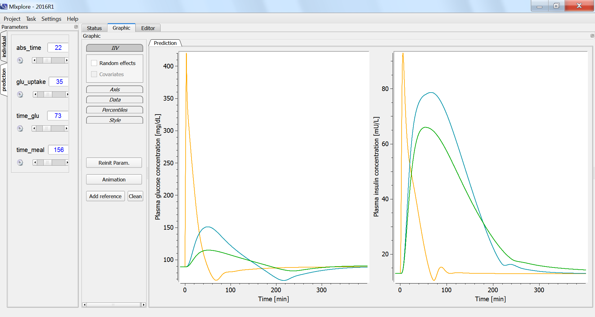
According to the specifications, given in the <RESULT> section, the graphics display the plasma glucose and insulin concentrations, fro the three glucose tolerance tests. In the figure below, the intravenous glucose test is in orange, the oral glucose in blue and the mixed meal in green. In case of an oral ingestion, the glucose concentration in the blood rises progressively. For the same total amount of glucose, the appearance of glucose in the blood is slower in the case of a mixed meal, compared to a glucose solution:

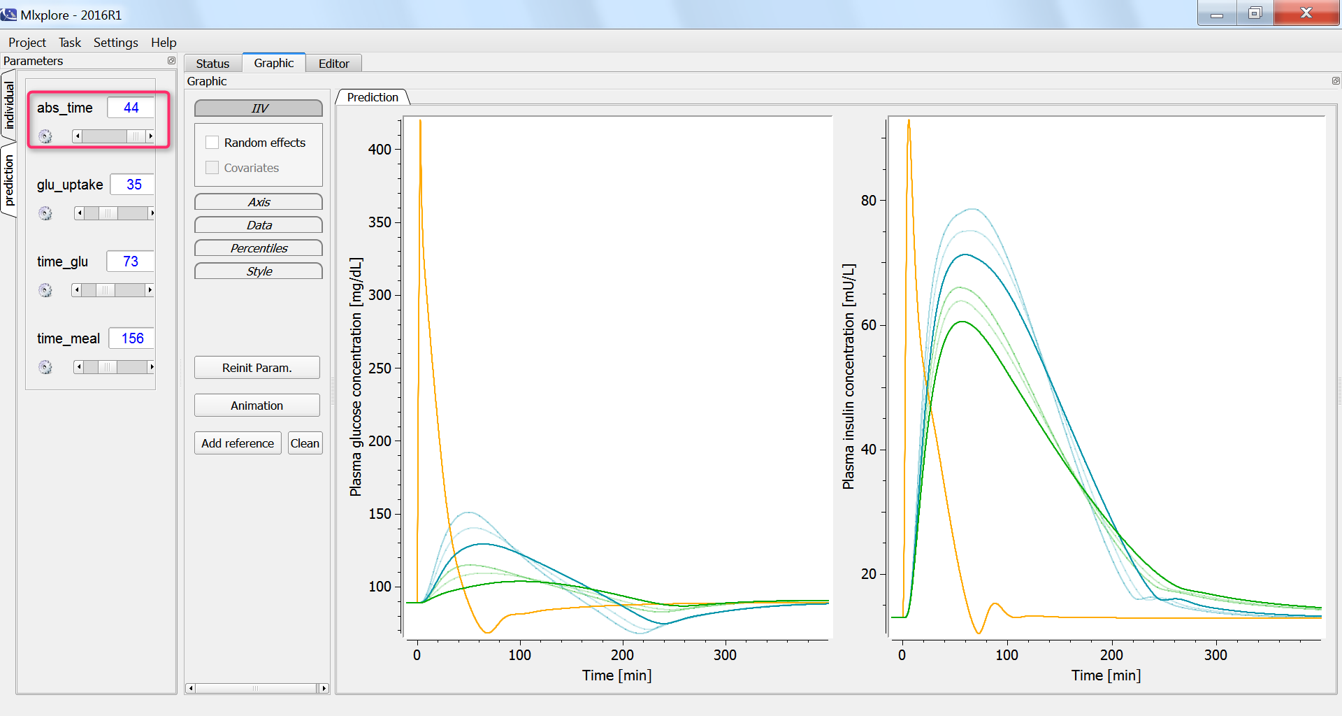
The influence of having a faster or slower characteristic time of absorption of glucose from the intestine into the blood (parameter abs_time) can be explored using the parameter slider:

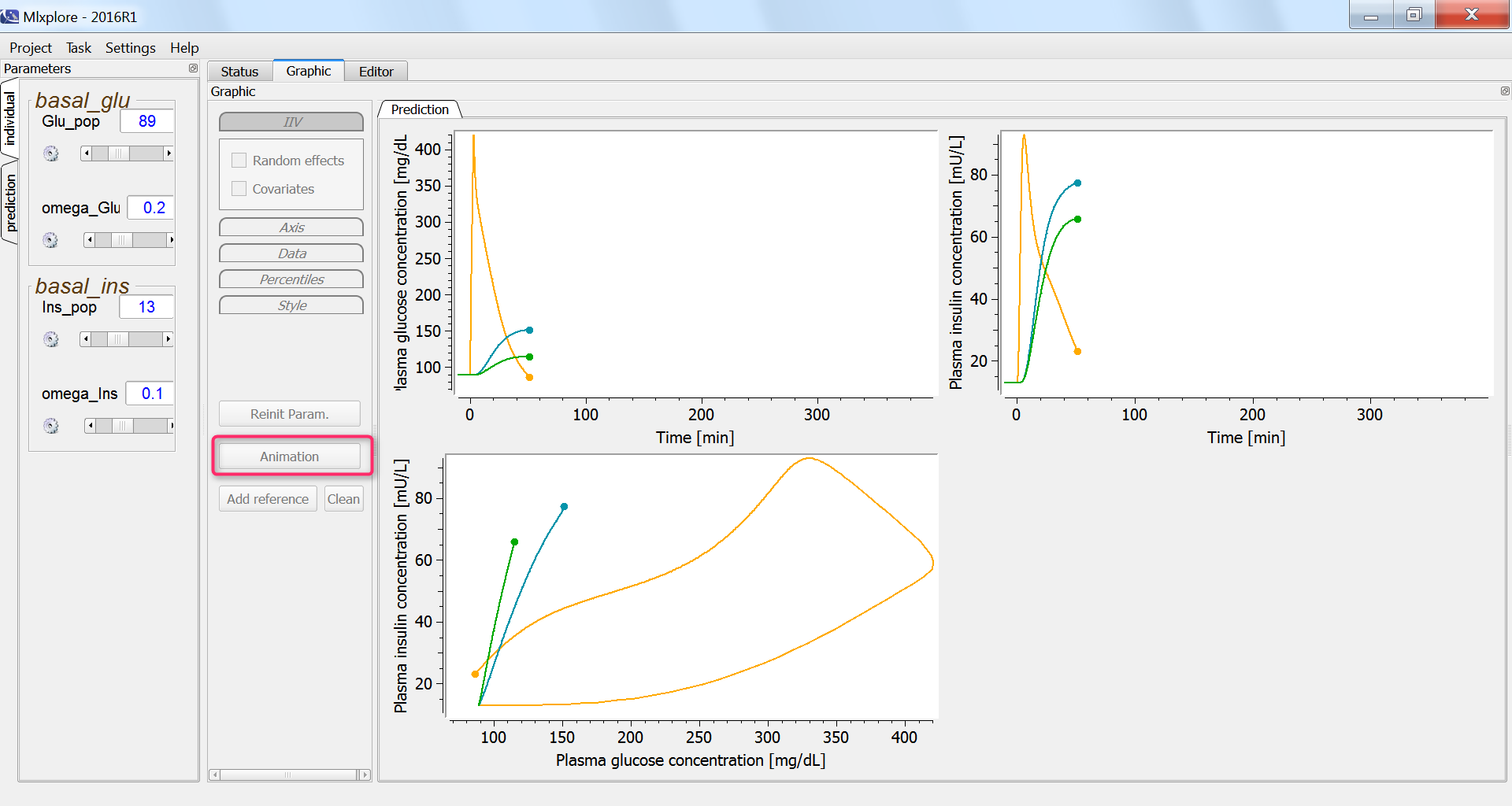
In all three cases, we expect that the glucose concentration increases first, triggering the increase in the insulin concentration. With the current display, this cannot be easily verified. We thus adapt the project file in order to output also the insulin concentration with respect to the glucose concentration, in the <RESULTS> section:

<RESULTS>
[GRAPHICS]
p1 = {y={venous_plasma_glucose}, ylabel='Plasma glucose concentration [mg/dL]', xlabel='Time [min]'}
p2 = {y={venous_plasma_insulin}, ylabel='Plasma insulin concentration [mU/L]', xlabel='Time [min]'}
p3 = {y={venous_plasma_insulin}, x={venous_plasma_glucose}, ylabel='Plasma insulin concentration [mU/L]', 
xlabel='Plasma glucose concentration [mg/dL]'}

In the graphics, we can use the “animation” button to see how glucose and insulin evolve over time. The hysteresis appears clearly, with first the rise of glucose and then that of insulin:

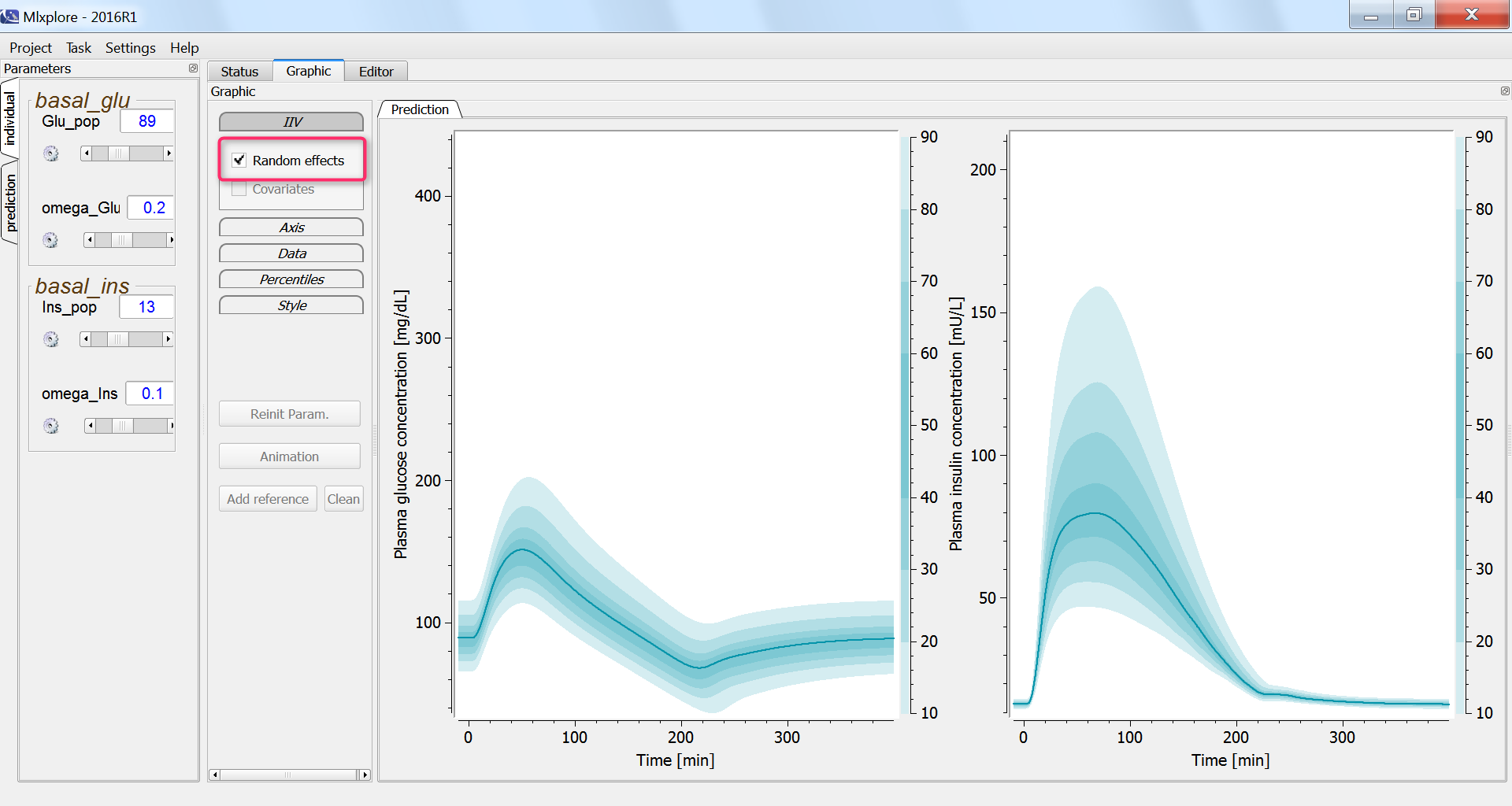
Finally, we assess the variability in the glucose and insulin concentrations after glucose uptake given that each individual has a slightly different basal glucose and insulin level:

Effect of physical exercice

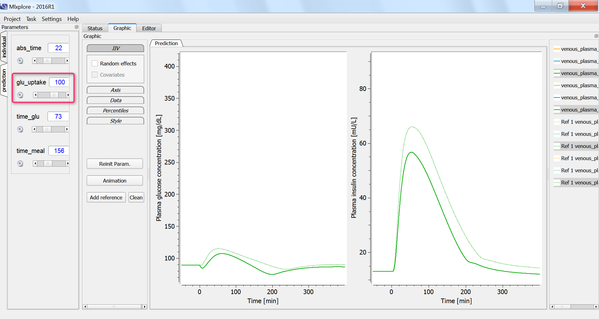
Next, we investigate the influence of physical exercice on the glucose concentration. During physical exercice, the glucose consumption by muscles increases. To capture this in the model, we increase the glucose uptake by the periphery compartment, which include muscles, from the initial 35 mg/min to 100 mg/min. As a consequence, the glucose and insulin concentrations increase less:

Conclusion

In this example a complex ODE-based PBPK model with 4 entities and 28 equations has been implemented. The real-time simulations permit to interactively explore the model behavior, even for large models.

In this case study, the effect of three glucose tolerance tests have been studied in conditions representing healthy humans. The model could be further adapted to simulate the expected response of diabetic individuals to the glucose tolerance tests.

Downloads

The Mlxplore project and model file can be downloaded here.